
Statistics [18]: Python [02] - t Test & F Test
Published:
test and
test, including 1 sample
test, 2 independent sample
test, paired sample
test and one-way and two-way ANOVA.
t Test
The examples in this part follows that from this post.
1 Sample t Test
scipy.stats.ttest_1samp(a, popmean, axis=0, nan_policy='propagate', alternative='two-sided')
This function tests if the population mean of data is likely to be equal to a given value. It returns the T statistic, and the p-value.
from scipy import stats
stats.ttest_1samp(data1['VIQ'], 0)
Result:
Ttest_1sampResult(statistic=30.088099970849328, pvalue=1.3289196468728067e-28)
With value 1.3289196468728067e-28, the null hypothesis is rejected.
2 Independent Samples t Test
scipy.stats.ttest_ind(a, b, axis=0, equal_var=True, nan_policy='propagate', permutations=None, random_state=None, alternative='two-sided', trim=0)
This is a test for the null hypothesis that 2 independent samples have identical average (expected) values. It returns the T statistic, and the p-value.
female_viq = data1[data1['Gender'] == 'Female']['VIQ']
male_viq = data1[data1['Gender'] == 'Male']['VIQ']
stats.ttest_ind(female_viq, male_viq)
Result:
Ttest_indResult(statistic=-0.7726161723275011, pvalue=0.44452876778583217)
With value 0.44452876778583217, the difference of the two samples is not significant.
Alternately, we can also use the non-parametric method mannwhitneyu().
scipy.stats.mannwhitneyu(x, y, use_continuity=True, alternative='two-sided', axis=0, method='auto', *, nan_policy='propagate')
Paired Samples t Test
scipy.stats.ttest_rel(a, b, axis=0, nan_policy='propagate', alternative='two-sided')
This is a test for the null hypothesis that two related or repeated samples have identical average (expected) values. It returns the T statistic, and the p-value.
stats.ttest_rel(data['FSIQ'], data['PIQ'])
Result:
Ttest_relResult(statistic=1.7842019405859857, pvalue=0.08217263818364236)
With value 0.08217263818364236, the difference of the two samples is not very significant.
Alternately, we can also use the non-parametric method wilcoxon().
scipy.stats.wilcoxon(x, y=None, zero_method='wilcox', correction=False, alternative='two-sided', mode='auto', *, axis=0, nan_policy='propagate')
One-Way ANOVA
The example in this part is borrowed from this post.
Data
A,B,C,D
25,45,30,54
30,55,29,60
28,29,33,51
36,56,37,62
29,40,27,73
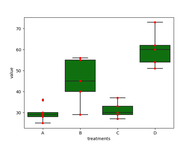
Here, there are four treatments (A, B, C, and D), the purpose is to test whether there are significant differences of the four treatments.
import pandas as pd
data = pd.read_csv('onewayanova.txt',sep=',')
# reshape the dataframe
dataMelt = data.melt(var_name='treatment')
Plot
import matplotlib.pyplot as plt
import seaborn as sns

ax = sns.boxplot(x='treatments', y='value', data=dataMelt, color='green')
ax = sns.swarmplot(x="treatments", y="value", data=dataMelt, color='red')
plt.show()
ANOVA Analysis
The simple way is to use scipy.stats.f_oneway(*samples, axis=0) from scipy.stats.
The one-way ANOVA tests the null hypothesis that two or more groups have the same population mean. The test is applied to samples from two or more groups, possibly with differing sizes. It returns the F statistic, and the p-value.
import scipy.stats as stats
fvalue, pvalue = stats.f_oneway(df['A'], df['B'], df['C'], df['D'])
print(fvalue, pvalue)
Result:
17.492810457516338 2.639241146210922e-05
Alternately, we can use statsmodels.formula.api.ols from statsmodels module to get ANOVA table as R like output.
import statsmodels.api as sm
from statsmodels.formula.api import ols

model = ols('value ~ C(treatments)', data=dataMelt).fit()
print(model.summary())
Result:
 OLS Regression Results
==============================================================================
Dep. Variable:                  value   R-squared:                       0.766
Model:                            OLS   Adj. R-squared:                  0.723
Method:                 Least Squares   F-statistic:                     17.49
Date:                Fri, 04 Mar 2022   Prob (F-statistic):           2.64e-05
Time:                        12:13:15   Log-Likelihood:                -66.643
No. Observations:                  20   AIC:                             141.3
Df Residuals:                      16   BIC:                             145.3
Df Model:                           3
Covariance Type:            nonrobust
======================================================================================
                         coef    std err          t      P>|t|      [0.025      0.975]
--------------------------------------------------------------------------------------
Intercept             29.6000      3.387      8.738      0.000      22.419      36.781
C(treatments)[T.B]    15.4000      4.791      3.215      0.005       5.244      25.556
C(treatments)[T.C]     1.6000      4.791      0.334      0.743      -8.556      11.756
C(treatments)[T.D]    30.4000      4.791      6.346      0.000      20.244      40.556
==============================================================================
Omnibus:                        0.549   Durbin-Watson:                   2.629
Prob(Omnibus):                  0.760   Jarque-Bera (JB):                0.020
Skew:                          -0.057   Prob(JB):                        0.990
Kurtosis:                       3.105   Cond. No.                         4.79
==============================================================================

Warnings:
[1] Standard Errors assume that the covariance matrix of the errors is correctly specified.
To obtain ANOVA table, use the anova_lm(), which can be referenced here.
anova_table = sm.stats.anova_lm(model, typ=2)
anova_table
Result:
                sum_sq    df         F    PR(>F)
C(treatments)  3010.95   3.0  17.49281  0.000026
Residual        918.00  16.0       NaN       NaN
With value 0.000026, the differences can be considered as significant.
Post-Hoc Analysis
The post-hoc analysis is used to see differences between specific groups. We can use bioinfokit to perform the post-hoc analysis using Tukey HSD for equal sample size and Tukey-Kramer for unequal sample sizes. (Document)
bioinfokit.analys.stat.tukey_hsd(df, res_var, xfac_var, anova_model, phalpha, ss_typ)
from bioinfokit.analys import stat
res = stat()
res.tukey_hsd(df=dataMelt, res_var='value', xfac_var='treatments', anova_model='value ~ C(treatments)')
print(res.tukey_summary)
Result:
  group1 group2  Diff      Lower      Upper   q-value   p-value
0      A      B  15.4   1.692871  29.107129  4.546156  0.025070
1      A      C   1.6 -12.107129  15.307129  0.472328  0.900000
2      A      D  30.4  16.692871  44.107129  8.974231  0.001000
3      B      C  13.8   0.092871  27.507129  4.073828  0.048178
4      B      D  15.0   1.292871  28.707129  4.428074  0.029578
5      C      D  28.8  15.092871  42.507129  8.501903  0.001000
We can see that except A-C pair, all the others show significant results.
Test ANOVA Assumptions
Shapiro-Wilk test can be used to check the normal distribution of residuals.
w, pvalue = stats.shapiro(model.resid)
print(w, pvalue)
Result:
0.9685019850730896 0.7229772806167603
With value 0.7229772806167603, we can conclude that the data are from normal distribution.
As the distribution is normal, Bartlett’s test can be used to check the Homogeneity of variances.
w, pvalue = stats.bartlett(data['A'], data['B'], data['C'], data['D'])
print(w, pvalue)
Result:
5.687843565012841 0.1278253399753447
With value 0.1278253399753447, we can conclude that the treatments have equal variances.
When the distribution is not normal, Levene’s test can be used to check the Homogeneity of variances.
res = stat()
res.levene(df=dataMelt, res_var='value', xfac_var='treatments')
res.levene_summary
Result:
                 Parameter   Value
0      Test statistics (W)  1.9220
1  Degrees of freedom (Df)  3.0000
2                  p value  0.1667
Two-Way ANOVA
Data
Genotype,1_year,2_year,3_year
A,1.53,4.08,6.69
A,1.83,3.84,5.97
A,1.38,3.96,6.33
B,3.6,5.7,8.55
B,2.94,5.07,7.95
B,4.02,7.2,8.94
C,3.99,6.09,10.02
C,3.3,5.88,9.63
C,4.41,6.51,10.38
D,3.75,5.19,11.4
D,3.63,5.37,9.66
D,3.57,5.55,10.53
E,1.71,3.6,6.87
E,2.01,5.1,6.93
E,2.04,6.99,6.84
F,3.96,5.25,9.84
F,4.77,5.28,9.87
F,4.65,5.07,10.08
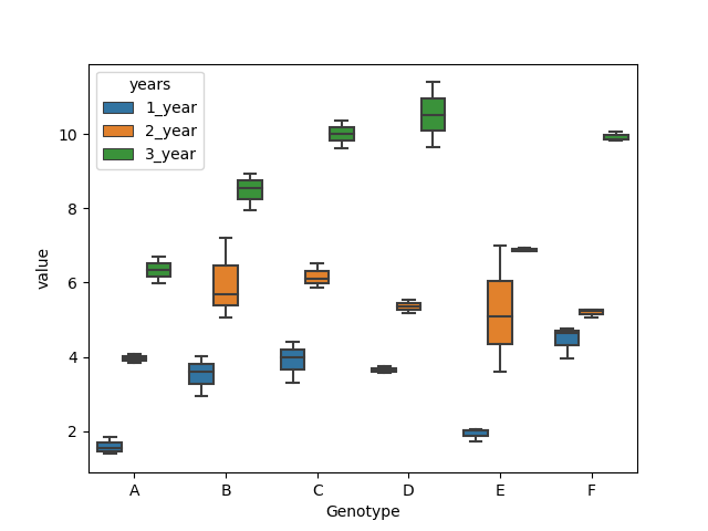
Here, there are 6 genotypes (A, B, C, D ,E and F) and three years, the purpose is to test how genotypes and years affects the yields of plants.
import pandas as pd
data = pd.read_csv('twowayanova.txt',sep=',')
# reshape the dataframe
dataMelt = data.melt(id_vars=['Genotype'], value_vars=['1_year', '2_year', '3_year'], var_name='years')
Plot
import matplotlib.pyplot as plt
import seaborn as sns

sns.boxplot(x="Genotype", y="value", hue="years", data=dataMelt)
ANOVA Analysis
import statsmodels.api as sm
from statsmodels.formula.api import ols
model = ols('value ~ C(Genotype) + C(years) + C(Genotype):C(years)', data=dataMelt).fit()
anova_table = sm.stats.anova_lm(model, typ=2)
anova_table
Result:
                          sum_sq    df           F        PR(>F)
C(Genotype)            58.551733   5.0   32.748581  1.931655e-12
C(years)              278.925633   2.0  390.014868  4.006243e-25
C(Genotype):C(years)   17.122967  10.0    4.788525  2.230094e-04
Residual               12.873000  36.0         NaN           NaN
The values suggest that the differences are significant.
Post-Hoc Analysis
from bioinfokit.analys import stat
res = stat()
# for main effect Genotype
res.tukey_hsd(df=dataMelt, res_var='value', xfac_var='Genotype', anova_model='value ~ C(Genotype) + C(years) + C(Genotype):C(years)')
res.tukey_summary
Result:
   group1 group2      Diff     Lower     Upper    q-value   p-value
0       A      B  2.040000  1.191912  2.888088  10.234409  0.001000
1       A      C  2.733333  1.885245  3.581421  13.712771  0.001000
2       A      D  2.560000  1.711912  3.408088  12.843180  0.001000
3       A      E  0.720000 -0.128088  1.568088   3.612145  0.135306
4       A      F  2.573333  1.725245  3.421421  12.910072  0.001000
5       B      C  0.693333 -0.154755  1.541421   3.478361  0.163609
6       B      D  0.520000 -0.328088  1.368088   2.608771  0.453066
7       B      E  1.320000  0.471912  2.168088   6.622265  0.001000
8       B      F  0.533333 -0.314755  1.381421   2.675663  0.425189
9       C      D  0.173333 -0.674755  1.021421   0.869590  0.900000
10      C      E  2.013333  1.165245  2.861421  10.100626  0.001000
11      C      F  0.160000 -0.688088  1.008088   0.802699  0.900000
12      D      E  1.840000  0.991912  2.688088   9.231036  0.001000
13      D      F  0.013333 -0.834755  0.861421   0.066892  0.900000
14      E      F  1.853333  1.005245  2.701421   9.297928  0.001000
# for main effect years
res.tukey_hsd(df=d_melt, res_var='value', xfac_var='years', anova_model='value ~ C(Genotype) + C(years) + C(Genotype):C(years)')
res.tukey_summary
Result:
   group1  group2      Diff     Lower     Upper    q-value  p-value
0  1_year  2_year  2.146667  1.659513  2.633821  15.230432    0.001
1  1_year  3_year  5.521667  5.034513  6.008821  39.175794    0.001
2  2_year  3_year  3.375000  2.887846  3.862154  23.945361    0.001
# for interaction effect between genotype and years
res.tukey_hsd(df=dataMelt, res_var='value', xfac_var=['Genotype','years'], anova_model='value ~ C(Genotype) + C(years) + C(Genotype):C(years)')
res.tukey_summary.head()
Result:
          group1       group2  Diff     Lower     Upper    q-value   p-value
0    (A, 1_year)  (A, 2_year)  2.38  0.548861  4.211139   6.893646  0.002439
1    (A, 1_year)  (A, 3_year)  4.75  2.918861  6.581139  13.758326  0.001000
2    (A, 1_year)  (B, 1_year)  1.94  0.108861  3.771139   5.619190  0.028673
3    (A, 1_year)  (B, 2_year)  4.41  2.578861  6.241139  12.773520  0.001000
4    (A, 1_year)  (B, 3_year)  6.90  5.068861  8.731139  19.985779  0.001000
..           ...          ...   ...       ...       ...        ...       ...
148  (E, 3_year)  (F, 2_year)  1.68 -0.151139  3.511139   4.866103  0.102966
149  (E, 3_year)  (F, 3_year)  3.05  1.218861  4.881139   8.834294  0.001000
150  (F, 1_year)  (F, 2_year)  0.74 -1.091139  2.571139   2.143402  0.900000
151  (F, 1_year)  (F, 3_year)  5.47  3.638861  7.301139  15.843799  0.001000
152  (F, 2_year)  (F, 3_year)  4.73  2.898861  6.561139  13.700396  0.001000

[153 rows x 7 columns]
Test ANOVA Assumptions
Shapiro-Wilk test can be used to check the normal distribution of residuals.
w, pvalue = stats.shapiro(res.anova_model_out.resid)
print(w, pvalue)
Rersult:
0.8978845477104187 0.00023986827000044286
As the distribution is not normal, Levene’s test can be used to check the Homogeneity of variances.
res = stat()
res.levene(df=dataMelt, res_var='value', xfac_var=['Genotype', 'years'])
res.levene_summary
Result:
                 Parameter    Value
0      Test statistics (W)   1.6849
1  Degrees of freedom (Df)  17.0000
2                  p value   0.0927
With value 0.0927, we can conclude that the samples have equal variances.
Table of Contents
- Probability vs Statistics
- Shakespear’s New Poem
- Some Common Discrete Distributions
- Some Common Continuous Distributions
- Statistical Quantities
- Order Statistics
- Multivariate Normal Distributions
- Conditional Distributions and Expectation
- Problem Set [01] - Probabilities
- Parameter Point Estimation
- Evaluation of Point Estimation
- Parameter Interval Estimation
- Problem Set [02] - Parameter Estimation
- Parameter Hypothesis Test
- t Test
- Chi-Squared Test
- Analysis of Variance
- Summary of Statistical Tests
- Python [01] - Data Representation
- Python [02] - t Test & F Test
- Python [03] - Chi-Squared Test
- Experimental Design
- Monte Carlo
- Variance Reducing Techniques
- From Uniform to General Distributions
- Problem Set [03] - Monte Carlo
- Unitary Regression Model
- Multiple Regression Model
- Factor and Principle Component Analysis
- Clustering Analysis
- Summary
Comments