Statistics [23]: Monte Carlo

4 minute read

Published: January 23, 2021

Monte Carlo (MC) technique is a numerical method that makes use of random numbers to solve mathematical problems for which an analytical solution is not known.

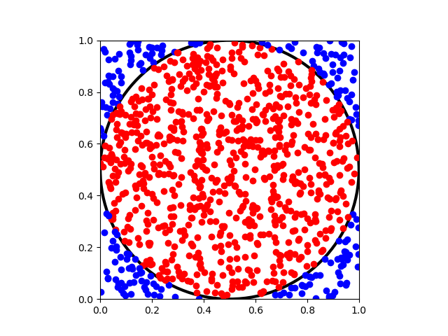
A Simple Example: Estimating Pi

Assume we have a circle $C$ with radius $r = 0.5$ inscribed within a square $S$ . The area ratio would be

$\dfrac{A_{C}}{A_{S}} = \dfrac{\pi r^2}{4r^2} = \dfrac{\pi}{4 }$

To determine $\pi$ , we can randomly select $n$ points in the square. Suppose $m$ points fall within the circle, we can then approximate the ratio by

$\dfrac{A_{C}}{A_{S}}=\dfrac{\pi}{4 }\approx \dfrac{m}{n}$

Hence,

$\pi = \dfrac{4m}{n}$

Here is the Python code.

import numpy as np
import random
import math
import matplotlib.pyplot as plt

inCircle = 0
outCircle = 0

piValue = []

# number of trials
numTrial = 1

# number of points within each trial
numPoints = 1000

data = np.random.random([numPoints,2])

fig = plt.figure()

for trial in range(numTrial):
    for i in range(numPoints):
        if (data[i][0]-0.5)**2 + (data[i][1]-0.5)**2 <= 1/4:
            plt.plot(data[i][0],data[i][1],'ro')
            inCircle += 1
        else:
            plt.plot(data[i][0],data[i][1],'bo')
            outCircle += 1
        
    piValue.append(4*inCircle/(inCircle + outCircle))

# result
print(sum(piValue)/len(piValue))

# plot
plt.xlim(0, 1)
plt.ylim(0, 1)
ax = fig.add_subplot(1, 1, 1)
plt.gca().set_aspect('equal', adjustable='box')
circ = plt.Circle((0.5, 0.5), 0.5, color='k',fill=False, linewidth=3)
ax.add_patch(circ)
plt.show()

drawing

The Law of Large Numbers

Assume $X_1,X_2,...,X_n$ are $n$ independent samples from the same distribution with $E(X_1)=E(X_2)=\cdots=E(X_n)=\mu$ . Let

$\bar{X}_n = {\displaystyle \dfrac{1}{n}\sum_{i=1}^n(X_1 + X_2 + \cdots + X_n)}$

Then

$\lim_{n\to\infty}\bar{X}_n = \mu$

Further assume $var(X_i) = \sigma^2$ ,

$var(\bar{X}_n) = \dfrac{1}{n^2}var(X_1 + X_2 + \cdots + X_n) = \dfrac{n\sigma^2}{n^2} = \dfrac{\sigma^2}{n}$ .

Weak Law of Large Numbers (Khinchin’s Law)

For $\forall\varepsilon>0$ and $n\to\infty$ , there is

$\lim_{n\to\infty}P\left(|\bar{X}_n-\mu| < \varepsilon\right) = 1$

which states that the sample average converges in probability towards the expected value.

Weak Law of Large Numbers ( Kolmogorov’s Law)

For $n\to\infty$ , there is

$P\left(\lim_{n\to\infty}\bar{X}_n=\mu\right) = 1$

which states that the sample average converges almost surely towards the expected value.

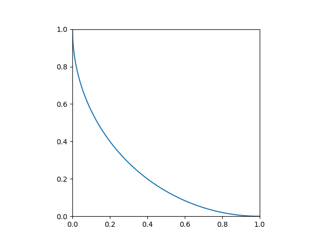
MC Integration

A Simple Example

Find ${\displaystyle \int_0^1\left(1 - \sqrt{x(2-x)}\right)}dx$ .

Firstly, let’s plot the curve of $x\sim 1 - \sqrt{x(2-x)}$ , the area under the curve would be $p$ .

drawing

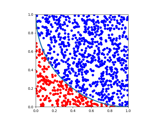
To determine $p$ , we can randomly select $n$ points in the square $[0,1]\times[0,1]$ . Suppose $m$ points fall under the curve, we can then approximate $p$ by

$p \approx \dfrac{m}{n}$

underCurve = 0
aboveCurve = 0

pValue = []

# number of trials
numTrial = 1

# number of points within each trial
numPoints = 1000

data = np.random.random([numPoints,2])

fig = plt.figure()

for trial in range(numTrial):
    for i in range(numPoints):
        x = data[i][0]
        y = 1 - np.sqrt(x*(2-x))
        if data[i][1] <= y:
            plt.plot(data[i][0],data[i][1],'ro')
            underCurve += 1
        else:
            plt.plot(data[i][0],data[i][1],'bo')
            aboveCurve += 1
        
    pValue.append(underCurve/(underCurve + aboveCurve))

# result
print(sum(pValue)/len(pValue))

x = np.linspace(0,1,1000)
y = 1 - np.sqrt(x*(2-x))
plt.plot(x,y,linewidth=3)
plt.xlim(0, 1)
plt.ylim(0, 1)
plt.gca().set_aspect('equal', adjustable='box')
plt.show()

drawing

General Case

Regular Domain of Integration

Find ${\displaystyle \int\int_{D}f(x)}dx$ , where the domain of integration is $D = [a,b]\times[c,d]$ .

We can randomly select $n$ points in $D$ , then

$E(f(X)) = \int\int_{D}f(x)\cdot\dfrac{1}{S_D}dx \approx \dfrac{1}{n}\sum_{k=1}^n f(x_k)$

Hence,

$\int\int_{D}f(x)dx \approx S_D\cdot\dfrac{f(x_1) + f(x_2) + \cdots + f(x_n)}{n}$

Non-Regular Domain of Integration

Find ${\displaystyle \int\int_{\Omega}f(x,y)}dxdy$ .

Similarly, we can randomly select $n$ points in $D$ that includes $\Omega$ . Suppose $m$ of the $n$ points fall within $D$ , then

$\int\int_{\Omega}f(x,y)dxdy = S_\Omega\int\int_{\Omega}f(x,y)\cdot\dfrac{1}{S_\Omega}dxdy = S_\Omega\cdot E(f(X,Y))$

Hence,

$\int\int_{\Omega}f(x,y)dxdy \approx \dfrac{m}{n}(b-a)(d-c)\dfrac{1}{m}\sum_{k=1}^m f(x_k,y_k) = \dfrac{(b-a)(d-c)}{n}\sum_{k=1}^m f(x_k,y_k)$

Example

In a shooting practice, assume the target is an ellipse with $a=1.2,b=0.8$ and the probability density function of hitting the target is $p(x,y) = \dfrac{1}{2\pi\sigma_x\sigma_y}\exp\left[-\dfrac{1}{2}\left(\dfrac{x^2}{\sigma_x^2}+ \dfrac{y^2}{\sigma_y^2}\right)\right]$ with $\sigma_x = 0.6, \sigma_y=0.4$ . Find $\int\int_{\Omega}p(x,y)dxdy$ , where $\Omega: \dfrac{x^2}{a^2}+ \dfrac{y^2}{b^2}\leq 1$ .

#
a = 1.2
b = 0.8
sx = 0.6
sy = 0.4

result = []

# number of trials
numTrial = 1

# number of points within each trial
numPoints = 1000

fig = plt.figure()

for trial in range(numTrial):
    z = 0
    for i in range(numPoints):
        x = np.random.random()*2*a-a
        y = np.random.random()*2*b-b       
        if x**2/a**2 + y**2/b**2 <= 1:
            plt.plot(x,y,'ro')
            u = np.exp(-0.5*(x**2/sx**2 + y**2/sy**2))
            z += u
        else:
            plt.plot(x,y,'bo')
    P = 4*a*b/numPoints*z/2/pi/sx/sy
    result.append(P)

# result
print(sum(result)/len(result))

# plot
mean = [0 , 0]
width = 2.4
height = 1.6
ell = mpl.patches.Ellipse(xy=mean, width=width, height=height, fill=False,linewidth=3)
ax = fig.add_subplot(1, 1, 1)

ax.add_patch(ell)
plt.xlim(-1.2, 1.2)
plt.ylim(-0.8, 0.8)
plt.gca().set_aspect('equal', adjustable='box')
plt.show()

drawing

Twitter Facebook LinkedIn

Chao Huang

Statistics [23]: Monte Carlo

A Simple Example: Estimating Pi

The Law of Large Numbers

Weak Law of Large Numbers (Khinchin’s Law)

Weak Law of Large Numbers ( Kolmogorov’s Law)

MC Integration

A Simple Example

General Case

Example

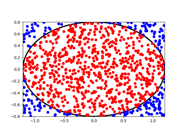
Table of Contents

Comments