Statistics [27]: Unitary Regression Model

5 minute read

Published: January 27, 2021

Basics of unitary regression, especially linear regression.

Review: Correlation

Correlation tells us whether the two variables are linearly dependent. If the two variables $X$ and $Y$ are independent, then $corr(X,Y)=0$ ; however, if $corr(X,Y)=0$ , it doesn’t necessarily mean that $X$ and $Y$ are independent, there might still be nonlinear relationships between the two variables.

For example, $X\sim N(0,1), Y=X^2$ , $X$ and $Y$ are obviously not independent. However,

$cov(X,Y) = cov(X,X^2) = E(X^3) - E(X)E(X^2) = 0$

It doesn’t mean that $X$ and $Y$ are independent, it only says that $X$ and $Y$ are linearly independent.

$corr(X,Y)=\pm 1$ if and only if $X$ and $Y$ are lienarly dependent almost everywhere. That is

$P(Y = aX+) = 1$

Least Square

Suppose the independent variable is $X$ and the dependent variable is $Y$ . The objective of linear fitting is to find a linear relationship between $X$ and $Y$ such that $\hat{Y}_i = b_1X_i + b_0$ . Residual is defined as the difference between the actual value and the fitted value, that is $e_i = Y_i-\hat{Y}_i$ .

Least square is to choose $b_0$ and $b_1$ to minimize $\sum_{i=1}^Ne_i^2$ , that is

$L(b_0,b_1) = \min \sum_{i=1}^N(y_i-(b_0+ b_1x_i))^2$

Differentiate $L(b_0,b_1)$ with respect to $b_0$ and $b_1$ respectively, we have

$\sum_{i=1}^N(y_i - (b_0+ b_1x_i)) = 0 \Rightarrow b_0 = \dfrac{\sum_{i=1}^Ny_i - \sum_{i=1}^Nx_ib_1}{N}$

$\sum_{i=1}^N[(y_i - (b_0+ b_1x_i))x_i] = 0 \Rightarrow b_1 = \dfrac{\sum_{i=1}^Nx_i\sum_{i=1}^Ny_i - N\sum_{i=1}^N(x_iy_i)}{\left(\sum_{i=1}^Nx_i\right)^2 - N\sum_{i=1}^Nx_i^2}$

Thus,

$b_1 = \dfrac{\sum_{i=1}^N(x_i-\bar{x})(y_i-\bar{y})}{\sum_{i=1}^N(x_i-\bar{x})^2} = \dfrac{S_{XY}}{S_X^2}=r_{xy}\cdot\dfrac{S_y}{S_x}, \ \ b_0 = \bar{y} - b_1\bar{x}$

Analysis of Variance

$\sum_{i=1}^N(y_i-\bar{y})^2 = \sum_{i=1}^N(y_i-\hat{y}_i) + 2\sum_{i=1}^N(y_i-\hat{y}_i)(\hat{y}_i - \bar{y}) + \sum_{i=1}^N(\hat{y}_i - \bar{y})^2$

where

$\sum_{i=1}^N(y_i-\hat{y}_i)(\hat{y}_i - \bar{y}) = \sum_{i-1}^Ne_i\hat{y}_i - \bar{y}\sum_{i=1}^Ne_i = 0$

Therefore,

$\sum_{i=1}^N(y_i-\bar{y})^2 = \sum_{i=1}^N(y_i-\hat{y}_i) + \sum_{i=1}^N(\hat{y}_i - \bar{y})^2$

where

$\sum_{i=1}^N(y_i-\bar{y})^2$ is the total sum of squares (TSS)
$\sum_{i=1}^N(\hat{y}_i - \bar{y})^2$ is the regression sum of squares (RegSS)
$\sum_{i=1}^N(y_i-\hat{y}_i)^2$ is the residual sum of squares (RSS)

A good fitting has a big RegSS and a small RSS. If TSS = RegSS, the fitting is perfect. The goodness of fit is determined by the coefficient of determination $R^2$ ,

$R^2 = \dfrac{\text{RegSS}}{\text{TSS}} = 1 - \dfrac{\text{RSS}}{\text{TSS}}$

Simple Linear Regression Model

The linear regression model is usually expressed as

$Y = \beta_0 + \beta_1 X + \varepsilon$

where $\varepsilon \sim N(0,\sigma^2)$ is the error term.

The least square model $\hat{Y} = b_0+ b_1X$ is an approximation of this linear regression model, where

$b_0 \sim N\left(\beta_0, \sigma^2\left(\dfrac{1}{n}+ \dfrac{\bar{x}^2}{L_{XX}}\right)\right), b_1 \sim N\left(\beta_1,\dfrac{\sigma^2}{L_{XX}}\right)$

with $L_{XX} = {\displaystyle \sum_{i=1}^N(x_i-\bar{x})^2}$

To prove this,

$b_1 = \dfrac{\sum_{i=1}^N(x_i-\bar{x})(y_i-\bar{y})}{\sum_{i=1}^N(x_i-\bar{x})^2} = \dfrac{\sum_{i=1}^N(x_i-\bar{x})y_i}{\sum_{i=1}^N(x_i-\bar{x})^2} - \dfrac{\sum_{i=1}^N(x_i-\bar{x})\bar{y}}{\sum_{i=1}^N(x_i-\bar{x})^2}$

$= \dfrac{\sum_{i=1}^N(x_i-\bar{x})(\beta_0+\beta_1x_i+\varepsilon_i)}{\sum_{i=1}^N(x_i-\bar{x})^2} - \dfrac{\sum_{i=1}^N(x_i-\bar{x})(\beta_0 + \beta_1\bar{x})}{\sum_{i=1}^N(x_i-\bar{x})^2} = \dfrac{\sum_{i=1}^N(x_i-\bar{x})(\beta_1x_i - \beta_1\bar{x} + \varepsilon_i)}{\sum_{i=1}^N(x_i-\bar{x})^2}$

$= \dfrac{\beta_1\sum_{i=1}^N(x_i-\bar{x})^2}{\sum_{i=1}^N(x_i-\bar{x})^2} + \dfrac{\sum_{i=1}^N(x_i-\bar{x})\varepsilon_i}{\sum_{i=1}^N(x_i-\bar{x})^2} = \beta_1 + \dfrac{\sum_{i=1}^N(x_i-\bar{x})\varepsilon_i}{\sum_{i=1}^N(x_i-\bar{x})^2}$

Hence,

$E(b_1) = \beta_1$

$var(b_1)= var\left(\dfrac{\sum_{i=1}^N(x_i-\bar{x})\varepsilon_i}{\sum_{i=1}^N(x_i-\bar{x})^2}\right) = \sum_{i=1}^N\left(\dfrac{x_i-\bar{x}}{\sum_{i=1}^N(x_i-\bar{x})^2}\right)^2\sigma^2 = \dfrac{\sigma^2}{\sum_{i=1}^N(x_i-\bar{x})^2} = \dfrac{\sigma^2}{L_{XX}}$

With $b_1$ ,

$b_0 = \bar{y} - b_1\bar{x} = \beta_0 + \beta_1\bar{x} + \bar{\varepsilon} - b_1\bar{x}$

Therefore,

$E(b_0) = \beta_0$

$var(b_0) = var\left(\bar{\varepsilon} - b_1\bar{x}\right) = \dfrac{var(\varepsilon)}{n}+ \bar{x}^2var(b_1) = \sigma^2\left(\dfrac{1}{n}+ \dfrac{\bar{x}^2}{L_{XX}}\right)$

Properties

Least square estimation has the following properties:

$b_0 \sim N\left(\beta_0, \sigma^2\left(\dfrac{1}{n}+ \dfrac{\bar{x}^2}{(n-1)s_x^2}\right)\right)$
$b_1 \sim N\left(\beta_1, \dfrac{\sigma^2}{(n-1)s_x^2}\right)$
$\dfrac{\text{RSS}}{\sigma^2}\sim \chi^2(n-2)$ (number of parameters subtracted from the freedom, proved in the next post)
$\bar{y},b_1,\text{RSS}$ are mutually independent (?).

Significance Test

In practice, the lienar regression model $Y = \beta_0 + \beta_1 X + \varepsilon$ is only a hypothesis. Therefore, we need to test the significance of this hypothesis, which is

$H_0: \beta_1 = 0\ \ \ \ H_1: \beta_1 \neq 0$

If $H_0$ is rejected, we can conclude that $X$ and $Y$ have a linear relationship; otherwise, it means that there is no significant linear relationship between $X$ and $Y$ .

F-Test

When $\beta_1$ holds, $b_1\sim N\left(0,\dfrac{\sigma^2}{L_{XX}}\right) \Rightarrow \dfrac{b_1\sqrt{L_{XX}}}{\sigma}\sim N(0,1)$

It can be proved that $\dfrac{\text{RegSS}}{\sigma^2}\sim \chi^2(1)$ , which will be proved in the next post.

As $\dfrac{\text{RSS}}{\sigma^2}\sim \chi^2(n-2)$ , we have,

$F = \dfrac{\text{RegSS}}{\text{RSS}/(n-2)} \sim F(1,n-2)$

t-Test

Since

$b_0 \sim N\left(\beta_0, \sigma^2\left(\dfrac{1}{n}+ \dfrac{\bar{x}^2}{L_{XX}}\right)\right), b_1 \sim N\left(\beta_1, \dfrac{\sigma^2}{L_{XX}}\right)$

When $\beta_0=0$ , we have

$\dfrac{\dfrac{b_0}{\sigma\sqrt{\dfrac{1}{n}+ \dfrac{\bar{x}^2}{L_{XX}}}}}{\sqrt{\dfrac{\text{RSS}}{\sigma^2}\Big/(n-2)}} = \dfrac{b_0}{\sqrt{\left(\dfrac{1}{n}+ \dfrac{\bar{x}^2}{L_{XX}}\right)\cdot\dfrac{\text{RSS}}{n-2}}} = \dfrac{b_0}{S_{\beta_0}}\sim t(n-2)$

When $\beta_1=0$ , we have

$\dfrac{\dfrac{b_0}{\dfrac{\sigma}{\sqrt{L_{XX}}}}}{\sqrt{\dfrac{\text{RSS}}{\sigma^2}\Big/(n-2)}} = \dfrac{b_0}{\sqrt{\dfrac{1}{L_{XX}}\cdot\dfrac{\text{RSS}}{n-2}}} = \dfrac{b_0}{S_{\beta_1}}\sim t(n-2)$

Hence, confidence interval of $\beta_0$ and $\beta_1$ are respectively

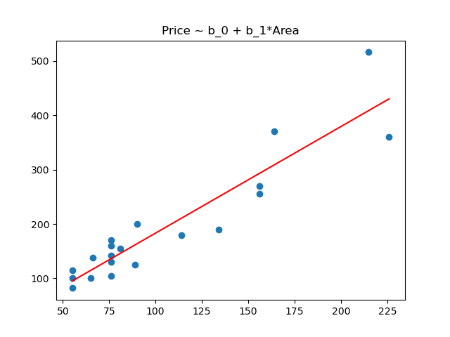
$\beta_0: \left[b_0-t_{\alpha\text{/}2}(n-2)\cdot S_{\beta_0}, b_0+ t_{\alpha\text{/}2}(n-2)\cdot S_{\beta_0}\right]$

$\beta_1: \left[b_1-t_{\alpha\text{/}2}(n-2)\cdot S_{\beta_1}, b_1+ t_{\alpha\text{/}2}(n-2)\cdot S_{\beta_1}\right]$

Example

Relationship between the area and price of houses.

	Area (m^2)	Price (10,000)
1	55	100
2	76	130
3	65	100
4	156	255
5	55	82
6	76	105
7	89	125
8	226	360
9	134	190
10	156	270
11	114	180
12	76	142
13	164	370
14	55	115
15	90	200
16	81	155
17	215	516
18	76	160
19	66	138
20	76	170

Linear regression using statsmodels.

import numpy as np
import pandas as pd
import matplotlib.pyplot as plt
import statsmodels.api as sm

data = np.array([[1,2,3,4,5,6,7,8,9,10,11,12,13,14,15,16,17,18,19,20],
                 [55,76,65,156,55,76,89,226,134,156,114,76,164,55,90,81,215,76,66,76],
                 [100,130,100,255,82,105,125,360,190,270,180,142,370,115,200,155,516,160,138,170]])
dataDF = pd.DataFrame(np.transpose(data),columns = ['Num','Area','Price'])  

Y = dataDF['Price']
X = dataDF['Area']
X = sm.add_constant(X)
model = sm.OLS(Y,X)
results = model.fit()

results.summary()

Results:

  OLS Regression Results                            
==============================================================================
Dep. Variable:                  Price   R-squared:                       0.857
Model:                            OLS   Adj. R-squared:                  0.849
Method:                 Least Squares   F-statistic:                     107.9
Date:                Tue, 08 Mar 2022   Prob (F-statistic):           4.94e-09
Time:                        12:13:11   Log-Likelihood:                -102.61
No. Observations:                  20   AIC:                             209.2
Df Residuals:                      18   BIC:                             211.2
Df Model:                           1                                         
Covariance Type:            nonrobust                                         
==============================================================================
                 coef    std err          t      P>|t|      [0.025      0.975]
------------------------------------------------------------------------------
const        -12.8246     22.046     -0.582      0.568     -59.142      33.493
Area           1.9607      0.189     10.390      0.000       1.564       2.357
==============================================================================
Omnibus:                        2.958   Durbin-Watson:                   0.845
Prob(Omnibus):                  0.228   Jarque-Bera (JB):                1.423
Skew:                           0.613   Prob(JB):                        0.491
Kurtosis:                       3.455   Cond. No.                         267.
==============================================================================

Warnings:
[1] Standard Errors assume that the covariance matrix of the errors is correctly specified.

x = [55,76,65,156,55,76,89,226,134,156,114,76,164,55,90,81,215,76,66,76]
x = np.sort(x)
y = results.params[1]*x + results.params[0]
plt.scatter(dataDF['Area'],dataDF['Price'])
plt.plot(x,y,'r')
plt.title('Price ~ b_0 + b_1*Area')
plt.show()

drawing

Linear regression using sklearn.

import numpy as np
from sklearn.linear_model import LinearRegression

x = np.array([55,76,65,156,55,76,89,226,134,156,114,76,164,55,90,81,215,76,66,76]).reshape((-1,1))
y = np.array([100,130,100,255,82,105,125,360,190,270,180,142,370,115,200,155,516,160,138,170])
model = LinearRegression(fit_intercept = True).fit(x,y)

Results:

model.coef_
# array([1.96072963])
model.intercept_
# -12.82464801609072
model.score(x,y)
# 0.8570804873379527

Prediction

Suppose $Y=\beta_0+ \beta_1X+ \varepsilon, \varepsilon\sim N(0,\sigma^2)$ , and the regression function is obtained from $(x_1,y_1),(x_2,y_2),...,(x_n,y_n)$ . Now fix $x_0$ such that $y_0 = \beta_1+ \beta_1 x_0+ \varepsilon_0$ , find the predicted value of $y_0$ along with its confidence interval.

It is easy to verify that $\hat{y}_0$ is an unbiased estimation with

$E(\hat{y}_0) = E(b_0+ b_1x_0) = \beta_0 + \beta_1 x_0 = E(y_0)$

Consider the distribution of $y_0-\hat{y}_0$ . Firstly,

$\hat{y}_0 = b_0+ b_1x_0 = \bar{y}-b_1\bar{x}+ b_1x_0 = \bar{y}+ b_1(x_0 - \bar{x})$

$var(\hat{y}_0) = \var(\bar{y}) + (x_0-\bar{x})^2var(b_1) = \sigma^2\left[\dfrac{1}{n}+ \dfrac{(x_0-\bar{x})^2}{L_{XX}}\right]$

Hence,

$\hat{y}_0\sim N\left(\beta_0+ \beta_1x_0, \sigma^2\left[\dfrac{1}{n}+ \dfrac{(x_0-\bar{x})^2}{L_{XX}}\right]\right), y_0 = N(\beta_0+ \beta_1x_0,\sigma^2)$

Therefore,

$y_0-\hat{y}_0\sim N\left(0,\sigma^2\left[1+ \dfrac{1}{n}+ \dfrac{(x_0-\bar{x})^2}{L_{XX}}\right]\right)$

Along with $\dfrac{\text{RSS}}{\sigma^2}\sim \chi^2(n-2)$ , we have

$\dfrac{\dfrac{y_0-\hat{y}_0}{\sigma\sqrt{1+ \dfrac{1}{n} + \dfrac{(x_0-\bar{x})^2}{L_{XX}}}}}{\sqrt{\dfrac{\text{RSS}}{\sigma^2(n-2)}}} = \dfrac{y_0-\hat{y}_0}{\sqrt{\left(1+ \dfrac{1}{n} + \dfrac{(x_0-\bar{x})^2}{L_{XX}}\right)\cdot\dfrac{\text{RSS}}{n-2}}}\sim t(n-2)$

Denote

$\delta(x_0) = t_{\alpha\text{/}2}(n-2)\cdot\sqrt{\left(1+ \dfrac{1}{n} + \dfrac{(x_0-\bar{x})^2}{L_{XX}}\right)\cdot\dfrac{\text{RSS}}{n-2}}$ ,

then the confidence interval of $y_0$ with significance level $\alpha$ is

$[\hat{y}_0-\delta(x_0),\hat{y}_0+ \delta(x_0)]$

Nonlinear Least Square

Suppose the joint density function of $(X,Y)$ is $p_{XY}(x,y)$ , $E(Y^2)$ exists. Let $\{\varphi(x) = E(Y|X=x), \ \ \text{when}\ \ p_X(x)>0 ; 0,\ \ \text{otherwise}\}$ , then $E[(Y-\varphi(X))^2] = \min_{\Phi}E[(Y-\Phi(X))^2]$

Proof. Consider the case of continuous variable,

$E[Y(\varphi(X)-\Phi(X))] = {\displaystyle int_{-\infty}^\infty\int_{-\infty}^\infty y\cdot(\varphi(x)-\Phi(x))p(x,y)dxddy = \int_{-\infty}^\infty(\varphi(x)-\Phi(x))dx\int_{-\infty}^\infty y p(x,y)dy}$

$= {\displaystyle \int_{-\infty}^\infty(\varphi(x)-\Phi(x))dx\int_{-\infty}^\infty y p(y|x)p_X(x)dy = \int_{-\infty}^\infty(\varphi(x)-\Phi(x))p_X(x)dx\int_{-\infty}^\infty y p(y|x)dy}$

$= {\displaystyle \int_{-\infty}^\infty(\varphi(x)-\Phi(x))p_X(x)\varphi(x)dx} = E[\varphi(X)(\varphi(X)-\Phi(X))]$

Hence,

$E[(Y-\Phi(X))^2] = E[(Y-\varphi(X) + \varphi(X) - \Phi(X))^2]$

$={\displaystyle E[(Y-\varphi(X))^2]+ E[(\varphi(X) - \Phi(X))^2]+ 2E[(Y-\varphi(X))(\varphi(X) - \Phi(X))]}$

$={\displaystyle E[(Y-\varphi(X))^2]+ E[(\varphi(X) - \Phi(X))^2]}$

This completes the proof.

The conditional expectation $E(Y|X)$ is a random variable dependent on $X$ , and it is the variable closest to $Y$ among all the variables that can be expressed by $X$ in the sense of least square.

Twitter Facebook LinkedIn

Chao Huang

Statistics [27]: Unitary Regression Model

Review: Correlation

Least Square

Analysis of Variance

Simple Linear Regression Model

Properties

Significance Test

F-Test

t-Test

Example

Prediction

Nonlinear Least Square

Table of Contents

Comments

	Area (m^2)	Price (10,000)
1	55	100
2	76	130
3	65	100
4	156	255
5	55	82
6	76	105
7	89	125
8	226	360
9	134	190
10	156	270
11	114	180
12	76	142
13	164	370
14	55	115
15	90	200
16	81	155
17	215	516
18	76	160
19	66	138
20	76	170

	Area (m^2)	Price (10,000)
1	55	100
2	76	130
3	65	100
4	156	255
5	55	82
6	76	105
7	89	125
8	226	360
9	134	190
10	156	270
11	114	180
12	76	142
13	164	370
14	55	115
15	90	200
16	81	155
17	215	516
18	76	160
19	66	138
20	76	170

	Area (m^2)	Price (10,000)
1	55	100
2	76	130
3	65	100
4	156	255
5	55	82
6	76	105
7	89	125
8	226	360
9	134	190
10	156	270
11	114	180
12	76	142
13	164	370
14	55	115
15	90	200
16	81	155
17	215	516
18	76	160
19	66	138
20	76	170