
Statistics [28]: Multiple Regression Model
Published:
The purpose of multiple regression model is to estimate the dependent variable (response variable) using multiple independent variables (explanatory variables).
Multiple Regression Model
Notation
Suppose there are subjects and data is collected from these subjects.
Data on the response variable is , which is represented by the column vector
.
Data on the explanatory variable
is
, which is represented by the
matrix
. The
row of
has data collected from the
subject and the
column of
has data for the
variable.
The Linear Model
The linear model is assumed to have the following form:
where .
In matrix notation, the model can be written as
The Intercept Term
The linear model stipulates that , which implies that when
, then
. This is not a reasonable assumption. Therefore, we usually add a intercept term to the model such that
Further, let , the above equation can be rewritten as
In matrix notation,
where now denotes the
matrix whose first column consists of all ones and
.
Estimation
Similar to the unitary regression model, is estimated by minimizing the residual sum of squares:
In matrix notation,
Using this notation, we have
Take partial derivatives with respect to yields
This gives linear equations for the
unknown
. The solution is denoted as
.
As lies in the column space of
, there is always solution(s). And if
is invertible, there will be a unique solution, which is given by
.
In fact, being invertible is equivalent to
. Thus when
is non-invertible,
. In other words, some columns of
is a linear combination of the other columns. Hence, some explanatory variables would be redundant.
Properties of the Estimator
Assume is invertible, the estimator
has the following properties.
Linearity
An estimator is said to be linear if it can be written as .
Unbiasedness
Covariance
where
Optimality
The Gaussian-Markov Theorem states that is the best linear unbiased estimator.
Fitted Values
Given the model, the fitted value can be written in matrix form as
which can be seen as the orthogonal projection of onto the column space of
.
Let such that
, the matrix
is called the Hat Matrix, which has the following properties:
- It is summetric
- It is idempotent,
With these properties, we can easily get
Residual
The residual of multiple regression
It can be verified that the residuals are orthogonal to the column space of , such that
As the first column of is all ones, it implies that
Because ,
is also orthogonal to
.
The expectation of is
The covariance matrix of is
Analysis of Variance
Similar to the unitary regression model,
with
As there are parameters in the model, we have
Thus, the confidence interval of is
The R-Squared is similarly defined as
and the adjusted R-Squared is defined as
If is high, it means that RSS is much smaller compared to TSS and hence the explanatory variables are really useful in predicting the response.
Expected Value of RSS
Firstly,
Hence,
As , we have
As , we get
Therefore, an unbiased estimator of is given by
This also implies that
Properties
We assume that . Equivalently,
are independent normals with mean 0 and variance
.
Distribution of
Since , we have
Distribution of
Since and
, we have
Distribution of Fitted Values
As and
, we have
Distribution of Residuals
As and
, we have
Distributions of RSS
As , we have
. And because
and
is symmetric and idempodent with rank
, we have
Independence of Residuals and
To prove the independence of and
, we can use the theorem below.
Theorem. Let and
be a fixed
matrix and
be a fixed
matrix. Then,
and
are independent if and only if
.
To prove the theorem, let . From the properties of the multivariate normal distribution,
. Hence,
and
are uncorrelated if and only if
.
Because and
, let
,
,
and
, then
Thus, we can conclude that and
are independent.
Simipliarly, as , let
, we have
Thus, we can also conclude that and
are independent.
Significance Test
F-Test
The null hypothesis would be
This means that the explanatory variable can be dropped from the linear model, let’s call this reduced model
, and let’s call the original model
It is always true that . If
is much smaller than
, it means that the explanatory variable
contributes a lot to the regression and hence cannot be dropped. Therefore, we can test
via the test statistic:
It can be proved that
Hence, the statistica would be
More generally, be the number of explanatory variables in
, we have
To prove this, denote the hat matrix in the two models by
and
, then
Assume , we should have
and
. Hence,
where and it is also idempotent since
Therefore, under the null hypothesis
We can thus obtain the statistic
Specially, when , the model becomes
. In this case,
and
. Thus the
statistic would be
And the value would be
t-Test
Under normality of the errors, we have , Hence,
where is the
diagonal entry of
. Under the null hypothesis when
, we have
This can be used to construct the statistic
value for testing
can be got by
Example
Data
Below is the medical test results of 14 diabetes, build a model to predict the blood sugar level based on other factors.
| Number | Cholesterol (mmol/L) | Triglycerides (mmol/L) | Insulin (muU/ml) | Glycated Hemoglobin (%) | Blood Sugar (mmol/L) |
|---|---|---|---|---|---|
| 1 | 5.68 | 1.90 | 4.53 | 8.20 | 11.20 |
| 2 | 3.79 | 1.64 | 7.32 | 6.90 | 8.80 |
| 3 | 6.02 | 3.56 | 6.95 | 10.80 | 12.30 |
| 4 | 4.85 | 1.07 | 5.88 | 8.30 | 11.60 |
| 5 | 4.60 | 2.32 | 4.05 | 7.50 | 13.40 |
| 6 | 6.05 | 0.64 | 1.42 | 13.60 | 18.30 |
| 7 | 4.90 | 8.50 | 12.60 | 8.50 | 11.10 |
| 8 | 5.78 | 3.36 | 2.96 | 8.00 | 13.60 |
| 9 | 5.43 | 1.13 | 4.31 | 11.30 | 14.90 |
| 10 | 6.50 | 6.21 | 3.47 | 12.30 | 16.00 |
| 11 | 7.98 | 7.92 | 3.37 | 9.80 | 13.20 |
| 12 | 11.54 | 10.89 | 1.20 | 10.50 | 20.00 |
| 13 | 5.84 | 0.92 | 8.61 | 6.40 | 13.30 |
| 14 | 3.84 | 1.20 | 6.45 | 9.60 | 10.40 |
Regression
Linear regression using statsmodels.
import numpy as np
import pandas as pd
import matplotlib.pyplot as plt
import statsmodels.api as sm

data = np.array([[5.68,3.79,6.02,4.85,4.60,6.05,4.90,5.78,5.43,6.50,7.98,11.54,5.84,3.84],
                 [1.90,1.64,3.56,1.07,2.32,0.64,8.50,3.36,1.13,6.21,7.92,10.89,0.92,1.20],
                 [4.53,7.32,6.95,5.88,4.05,1.42,12.60,2.96,4.31,3.47,3.37,1.20,8.61,6.45],
                 [8.20,6.90,10.8,8.30,7.50,13.6,8.50,8.00,11.3,12.3,9.80,10.50,6.40,9.60],
                 [11.2,8.80,12.3,11.6,13.4,18.3,11.1,13.6,14.9,16.0,13.20,20.0,13.3,10.4]])
dataDF = pd.DataFrame(np.transpose(data),columns = ['X1','X2','X3','X4','Y'])

Y = dataDF['Y']
X = dataDF[['X1','X2','X3','X4']]
X = sm.add_constant(X)
model = sm.OLS(Y,X)
results = model.fit()

results.summary()
Results:
                            OLS Regression Results
==============================================================================
Dep. Variable:                      Y   R-squared:                       0.797
Model:                            OLS   Adj. R-squared:                  0.707
Method:                 Least Squares   F-statistic:                     8.844
Date:                Wed, 09 Mar 2022   Prob (F-statistic):            0.00349
Time:                        21:23:23   Log-Likelihood:                -23.816
No. Observations:                  14   AIC:                             57.63
Df Residuals:                       9   BIC:                             60.83
Df Model:                           4
Covariance Type:            nonrobust
==============================================================================
                 coef    std err          t      P>|t|      [0.025      0.975]
------------------------------------------------------------------------------
const          3.1595      4.308      0.733      0.482      -6.587      12.906
X1             1.1329      0.492      2.304      0.047       0.021       2.245
X2            -0.2042      0.245     -0.833      0.427      -0.759       0.351
X3            -0.1349      0.237     -0.570      0.583      -0.670       0.400
X4             0.5345      0.257      2.080      0.067      -0.047       1.116
==============================================================================
Omnibus:                        2.606   Durbin-Watson:                   1.337
Prob(Omnibus):                  0.272   Jarque-Bera (JB):                1.114
Skew:                          -0.221   Prob(JB):                        0.573
Kurtosis:                       1.691   Cond. No.                         128.
==============================================================================

Warnings:
[1] Standard Errors assume that the covariance matrix of the errors is correctly specified.
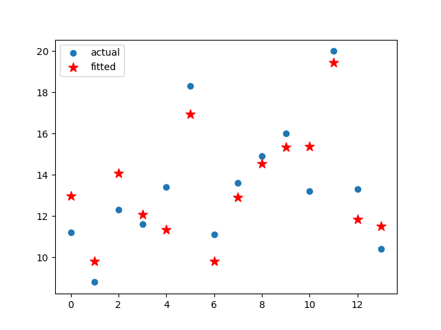
plt.scatter(range(len(Y)),Y,label='actual')
plt.scatter(range(len(Y)),results.fittedvalues,c="r",marker='*',label="fitted",s=10**2)
plt.legend()
plt.show()
An alternate way is to use functions provided in statsmodels.formula.api, which has the constant term by default.
###
from statsmodels.formula.api import ols
model = ols('Y ~ X1 + X2 + X3 + X4', data=dataDF).fit()
Results:
                            OLS Regression Results
==============================================================================
Dep. Variable:                      Y   R-squared:                       0.797
Model:                            OLS   Adj. R-squared:                  0.707
Method:                 Least Squares   F-statistic:                     8.844
Date:                Wed, 09 Mar 2022   Prob (F-statistic):            0.00349
Time:                        21:55:34   Log-Likelihood:                -23.816
No. Observations:                  14   AIC:                             57.63
Df Residuals:                       9   BIC:                             60.83
Df Model:                           4
Covariance Type:            nonrobust
==============================================================================
                 coef    std err          t      P>|t|      [0.025      0.975]
------------------------------------------------------------------------------
Intercept      3.1595      4.308      0.733      0.482      -6.587      12.906
X1             1.1329      0.492      2.304      0.047       0.021       2.245
X2            -0.2042      0.245     -0.833      0.427      -0.759       0.351
X3            -0.1349      0.237     -0.570      0.583      -0.670       0.400
X4             0.5345      0.257      2.080      0.067      -0.047       1.116
==============================================================================
Omnibus:                        2.606   Durbin-Watson:                   1.337
Prob(Omnibus):                  0.272   Jarque-Bera (JB):                1.114
Skew:                          -0.221   Prob(JB):                        0.573
Kurtosis:                       1.691   Cond. No.                         128.
==============================================================================

Warnings:
[1] Standard Errors assume that the covariance matrix of the errors is correctly specified.
Variable Selection
From the results, we can see that value of
and
are 0.426 and 0.583 respectively, meaning that their influence may not be that dignificant than
and
. Therefore, let’s do the regression again considering only
and
.
model = ols('Y ~ X1 + X4', data=dataDF).fit()
Results:
                            OLS Regression Results
==============================================================================
Dep. Variable:                      Y   R-squared:                       0.745
Model:                            OLS   Adj. R-squared:                  0.699
Method:                 Least Squares   F-statistic:                     16.07
Date:                Wed, 09 Mar 2022   Prob (F-statistic):           0.000545
Time:                        22:08:30   Log-Likelihood:                -25.420
No. Observations:                  14   AIC:                             56.84
Df Residuals:                      11   BIC:                             58.76
Df Model:                           2
Covariance Type:            nonrobust
==============================================================================
                 coef    std err          t      P>|t|      [0.025      0.975]
------------------------------------------------------------------------------
Intercept      1.8257      2.253      0.810      0.435      -3.133       6.784
X1             0.9517      0.255      3.729      0.003       0.390       1.513
X4             0.6358      0.237      2.686      0.021       0.115       1.157
==============================================================================
Omnibus:                        1.107   Durbin-Watson:                   1.652
Prob(Omnibus):                  0.575   Jarque-Bera (JB):                0.726
Skew:                           0.048   Prob(JB):                        0.695
Kurtosis:                       1.888   Cond. No.                         57.4
==============================================================================

Warnings:
[1] Standard Errors assume that the covariance matrix of the errors is correctly specified.
plt.scatter(range(len(Y)),Y,label='actual')
plt.scatter(range(len(Y)),results.fittedvalues,c="r",marker='*',label="fitted-full",s=10**2)
plt.scatter(range(len(Y)),model.fittedvalues,c="g",marker='h',label="fitted-reduced",s=10**2,alpha=0.5)
plt.legend()
plt.show()
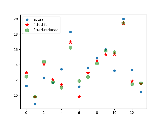
Table of Contents
- Probability vs Statistics
- Shakespear’s New Poem
- Some Common Discrete Distributions
- Some Common Continuous Distributions
- Statistical Quantities
- Order Statistics
- Multivariate Normal Distributions
- Conditional Distributions and Expectation
- Problem Set [01] - Probabilities
- Parameter Point Estimation
- Evaluation of Point Estimation
- Parameter Interval Estimation
- Problem Set [02] - Parameter Estimation
- Parameter Hypothesis Test
- t Test
- Chi-Squared Test
- Analysis of Variance
- Summary of Statistical Tests
- Python [01] - Data Representation
- Python [02] - t Test & F Test
- Python [03] - Chi-Squared Test
- Experimental Design
- Monte Carlo
- Variance Reducing Techniques
- From Uniform to General Distributions
- Problem Set [03] - Monte Carlo
- Unitary Regression Model
- Multiple Regression Model
- Factor and Principle Component Analysis
- Clustering Analysis
- Summary
Comments