Statistics [29]: Factor and Principle Component Analysis

17 minute read

Published: January 29, 2021

In practice, data may contain many variables, however, not all of them have significant influence on the results we want to analysis or predict. Factor analysis and principle component analysis are two basic methods that aim to reduce the dimension of the data to make it easier to understand and analyze.

Factor Analysis

Factor Analysis is a method for modeling observed variables, and their covariance structure, in terms of a smaller number of underlying unobservable (latent) “factors.”

Notations

Observabale variable (with $p$ traits):

$X = (X_1, X_2, ..., X_p)^T$

Common factors (with $m$ factors):

$f = (f_1, f_2, ..., f_m),\ \ m\ll p$

The factor model can be thought of as a series of multiple regressions:

$X_1 = \mu_1 + l_{11}f_1 + l_{12}f_2 + \cdots + l_{1m}f_m + \epsilon_1$

$X_2 = \mu_2 + l_{21}f_1 + l_{22}f_2 + \cdots + l_{2m}f_m + \epsilon_2$

$\vdots$

$X_p = \mu_1 + l_{p1}f_1 + l_{p2}f_2 + \cdots + l_{pm}f_m + \epsilon_p$

where $l_{ij}$ are called factor loadings.

In matrix form:

$X = \mu + Lf + \epsilon$

where

$\Lambda = \diag(\lambda_1,\lambda_2,...,\lambda_p), \ \ V = [v_1,v_2,...,v_p]$

Assumptions

Mean

$E(\epsilon_i) = 0, i=1,2,...,p$

$E(f_j) = 0, j=1,2,...,m$

Hence,

$E(X_i) = \mu_i, i=1,2,...,p$

Variance

$var(\epsilon_i) = \psi_i, i=1,2,...,p$ , where $\psi_i$ is the specific variance.

$var(f_j) = 1, j=1,2,...,m$

Correlation

$cov(f_i,f_j) = 0,\ \ \text{for}\ \ i\neq j$

$cov(\epsilon_i,\epsilon_j) = 0,\ \ \text{for}\ \ i\neq j$

$cov(\epsilon_i,f_j) = 0,\ \ \text{for}\ \ i=1,2,...,p; j=1,2,...,m$

Model Properties

$\sigma_i^2 = var(X_i) = E[(X_i-E(X_i))^2] = E[(l_{i1}f_1 + l_{i2}f_2 + \cdots + l_{im}f_m + \epsilon_i)^2] = \sum_{j=1}^ml_{ij}^2 + \psi_i$

where $\sum_{j=1}^ml_{ij}^2$ is called the communality of the variable $i$ .

$\sigma_{ij} = cov(X_i,X_j) = E[(X_i-E(X_i))(X_j-E(X_j))] = E[(l_{i1}f_1 + l_{i2}f_2 + \cdots + l_{im}f_m + \epsilon_i)(l_{j1}f_1 + l_{j2}f_2 + \cdots + l_{jm}f_m + \epsilon_j)] = \sum_{k=1}^ml_{ik}l_{jk}$

$cov(X_i,f_j) = l_{ij}$

In matrix form:

$\Sigma = LL^T + \Psi$

where $\Psi = \diag(\psi_1,\psi_2,...,\psi_p)$

As $\Sigma$ is a symmetric matrix, there are $\dfrac{p(p+ 1)}{2}$ parameters in total, which are to be approximated by $mp+ p$ parameters.

Principle Component Method

Let $X_i,i=1,2,...,n$ denote the samples, with

$X_i = (X_{i1},X_{i2},...,X_{ip})^T$

$S$ denotes the sample variance matrix,

$S = \dfrac{1}{n-1}{\displaystyle \sum_{i=1}^n(X_i-\bar{X})(X_i-\bar{X})^T}$

We have $p$ eigenvalues and $p$ eigenvectors for this matrix.

Eigenvalues: $\lambda_1,\lambda_2,...\lambda_p$

Eigenvectors: $v_1,v_2,...,v_p$

Then we can express the covariance matrix with eigenvalues and eigenfactors as

$S = V\Lambda V^T = {\displaystyle \sum_{i=1}^p\lambda_iv_iv_i^T}$

The idea behind the principal component method is to approximate this expression. Instead of summing from $1$ to $p$ , we sum from 1 to $m$ , ignoring the $p-m$ terms.

We can rewrite the covariance matrix as

$S \approx \sum_{i=1}^m\lambda_iv_iv_i^T = \sum_{i=1}^m\hat{l}_i\hat{l}_i^T, \hat{l}_i = (\hat{l}_{1i},\hat{l}_{2i},...,\hat{l}_{pi})^T$

This yields the estimator for the factor loadings:

$\hat{l}_{ij} = v_{ji}\sqrt{\lambda_j}\ \ \text{or}\ \ \hat{l}_{ji} = v_{ij}\sqrt{\lambda_i}$

To estimate the specific variances $\Psi$ , we only need to estimate the diagonal elements,

$\hat{\psi}_i = s_i^2 - \sum_{j=1}^m l_{ij}^2 = s_i^2 - {\displaystyle \sum_{j=1}^m\lambda_jv_{ji}^2}$

Maximum Likelihood Estimation Method

Using the Maximum Likelihood Estimation Method, we must assume that the data are independently sampled from a multivariate normal distribution with mean vector $\mu$ and covariance matrix of the form:

$\Sigma = LL^T + \Psi$

The maximum likelihood estimator for the mean vector $\mu$ , the factor loading matrix $L$ and the specific variance $\Psi$ are obtained by finding $\hat{\mu}$ , $\hat{L}$ and $\hat{\Psi}$ that maximize the maximize the log likelihood given by:

$l(\mu,L,\Psi) = -\dfrac{np}{2}\log 2\pi -\dfrac{n}{2}\log|LL^T+ \Psi| - \dfrac{1}{2}{\displaystyle \sum_{i=1}^n(X_i-\mu)^T(LL^T+ \Psi)^{-1}(X_i-\mu)}$

which can be obtained using the multivariate normal distribution given in this post.

Goodness of Fit

To assess goodness-of-fit, we use the Bartlett-Corrected Likelihood Ratio Test Statistic (link):

$X^2 = \left(n-1-\dfrac{2p+ 4m -5}{6}\right)\log\dfrac{\left|\hat{L}\hat{L}^T+ \Psi\right|}{|\hat{\Sigma}|}$

In the numerator we have the determinant of the fitted factor model for the variance-covariance matrix, and below, we have a sample estimate of the variance-covariance matrix assuming no structure where:

$\hat{\Sigma} = \dfrac{n-1}{n}S$

and $S$ is the sample covariance matrix.

If the factor model fits well then these two determinants should be about the same and you will get a small value for $X^2$ . Otherwise, $X^2$ would be large.

Under the null hypothesis that the factor model adequately describes the relationships among the variables, there is

$X^2\sim \chi^2((p^2-p-2pm)\text{/}2)$

where the degrees of freedom are the difference of unique parameters in the two models.

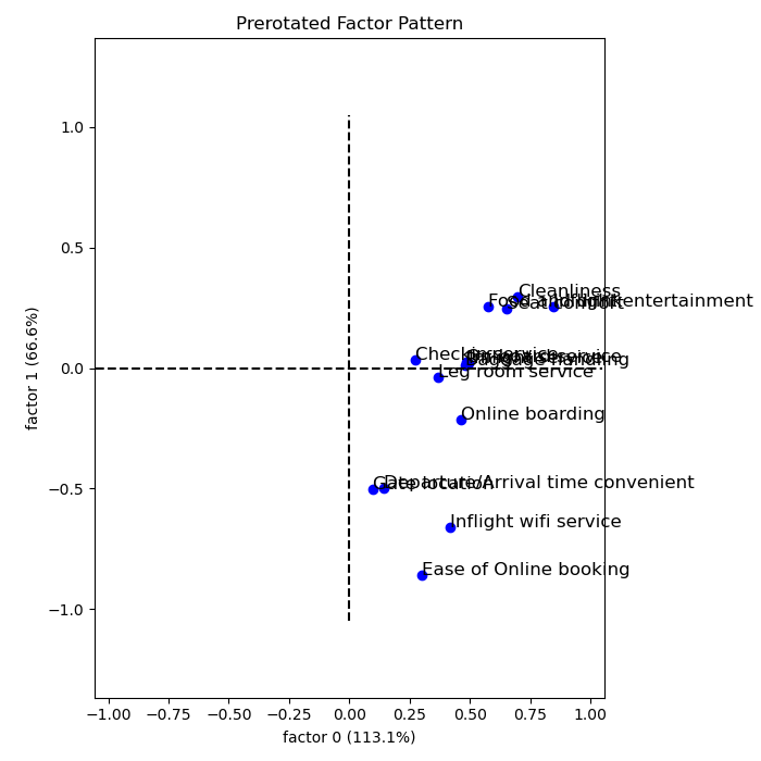
Factor Rotations

The problem with the analysis above is that some of the variables are highlighted by more than one factors, and some even indicate contradictory results. This does not provide a very clean, simple interpretation of the data. Ideally, each variable would appear as a significant contributer in one column (factor). This is the purpose of factor rotations.

Factor rotation is motivated by the fact that factor models are not unique. To see this, let $T$ be any $m\times m$ orthogonal matrix. We can write the factor model as:

$X=\mu + Lf + \epsilon =\mu + LTT^Tf + \epsilon = \mu + L^*f^* + \epsilon\ \ (L^*=LT, f^*=T^Tf)$

We can verify that the assumptions still hold under the trasform.

Varimax Rotation

Varimax rotation finds the rotation that maximizes the sum of the variances of the squared loadings, namely, find $T$ , such that

$V = {\displaystyle \dfrac{1}{p} \sum_{j=1}^m\left\{\sum_{i=1}^p(\tilde{l}_{ij}^*)^4 - \dfrac{1}{p}\left(\sum_{i=1}^p(\tilde{l}_{ij}^*)^2\right)^2\right\}}$

is maximized, where

$\tilde{l}_{ij}^* = \dfrac{\hat{l}_{ij}^*}{\hat{h}_i}$

and

$\hat{h}_i^2 = {\displaystyle \sum_{j=1}^m\hat{l}_{ij}^2}$

Estimation of Factor Scores

Given the factor model:

$Y_i = \mu + Lf_i + \epsilon_i, i=1,2,...,n$

estimate the vectors of factor scores

$f_1,f_2,...,f_n$

for each observation.

Ordinary Least Squares (OLS)

The factor scores is found by minimizing the sum of the residual squares:

$\epsilon_i^T\epsilon_i = (Y_i-\mu-Lf_i)^T(Y_i-\mu-Lf_i)$

Thus,

$\hat{f}_i = (L^TL)^{-1}L^T(Y_i-\mu)$

Weightead Least Squares (WLS)

The difference between WLS and OLS is that the squared residuals are divided by the specific variances $\psi$ . This is going to give more weight, in this estimation, to variables that have low specific variances.

The factor scores is found by minimizing the sum of the residual squares:

$\epsilon_i^T\Psi^{-1}\epsilon_i = (Y_i-\mu-Lf_i)^T\Psi^{-1}(Y_i-\mu-Lf_i)$

Thus,

$\hat{f}_i = (L^TL)^{-1}L^T\Psi^{-1}(Y_i-\mu)$

Example

Data

Here is an example using package factor_analyzer. Let repeat the example using statsmodel.

The dataset contains an airline passenger satisfaction survey, which has 25976 observations and 25 columns.

       Unnamed: 0     id  ... Arrival Delay in Minutes             satisfaction
             0  19556  ...                     44.0                satisfied
             1  90035  ...                      0.0                satisfied
             2  12360  ...                      0.0  neutral or dissatisfied
             3  77959  ...                      6.0                satisfied
             4  36875  ...                     20.0                satisfied
          ...    ...  ...                      ...                      ...
     25971  78463  ...                      0.0  neutral or dissatisfied
     25972  71167  ...                      0.0                satisfied
     25973  37675  ...                      0.0  neutral or dissatisfied
     25974  90086  ...                      0.0                satisfied
     25975  34799  ...                      0.0  neutral or dissatisfied

[25976 rows x 25 columns]

Here is a list of the 25 columns, where the columns 8 to 21 represent customers response on a scale of 1 to 5 to a survey evaluating different aspects of the flights.

['Unnamed: 0',
 'id',
 'Gender',
 'Customer Type',
 'Age',
 'Type of Travel',
 'Class',
 'Flight Distance',
 'Inflight wifi service',
 'Departure/Arrival time convenient',
 'Ease of Online booking',
 'Gate location',
 'Food and drink',
 'Online boarding',
 'Seat comfort',
 'Inflight entertainment',
 'On-board service',
 'Leg room service',
 'Baggage handling',
 'Checkin service',
 'Inflight service',
 'Cleanliness',
 'Departure Delay in Minutes',
 'Arrival Delay in Minutes',
 'satisfaction']

The first step of any factor analysis is to look at a correlation plot of all the variables to see if any variables are useless or too correlated with others.

import pandas as pd
import seaborn as sns
import matplotlib.pyplot as plt

data = pd.read_csv('airline.csv',sep=',')

c = data.corr()
ax = sns.heatmap(c,square=True)
ax.figure.subplots_adjust(bottom = 0.25)

drawing

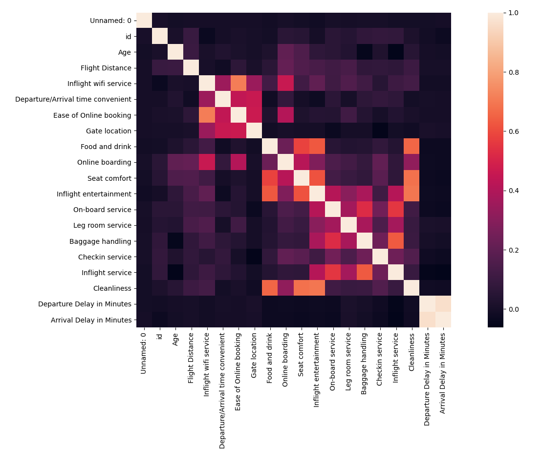
As “Departure Delay in Minutes” and the “Arrival Delay in Minutes” are highly correlated, remove one of the columns from the dataset.

data.drop(['Arrival Delay in Minutes'], axis=1, inplace=True)

Factor Analysis

class statsmodels.multivariate.factor.Factor(endog=None, n_factor=1, corr=None, method='pa', smc=True, endog_names=None, nobs=None, missing='drop')

Parameters
  endog: array_like
     Variables in columns, observations in rows. May be None if corr is not None.

  n_factor: int
    The number of factors to extract
    
  method: str
    The method to extract factors, currently must be either ‘pa’ for principal axis factor analysis or ‘ml’ for maximum likelihood estimation.

# 14 columns of the customers's responses to the survey
x =data[data.columns[8:22]] 
# set the number of factor as 3
results = sm.Factor(x,3).fit()

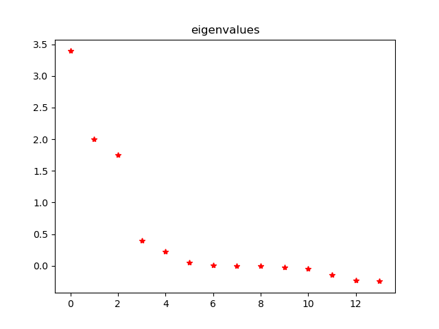
Eigenvalues:

results.eigenvals

Out[116]: 
array([ 3.39287070e+00,  1.99752234e+00,  1.74684264e+00,  4.03928420e-01,
        2.25980639e-01,  4.79457525e-02,  1.14410507e-02, -1.96191104e-03,
       -5.44379913e-03, -2.43802755e-02, -4.67822926e-02, -1.43716548e-01,
       -2.23380565e-01, -2.43630473e-01])

drawing

Communality：

results.communality

Out[124]: 
array([0.62136998, 0.26925258, 0.85027123, 0.27214144, 0.57158413,
       0.2980277 , 0.63998574, 0.78040315, 0.50684261, 0.25212025,
       0.5932482 , 0.10115273, 0.6385212 , 0.74231474])

drawing

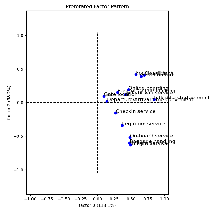
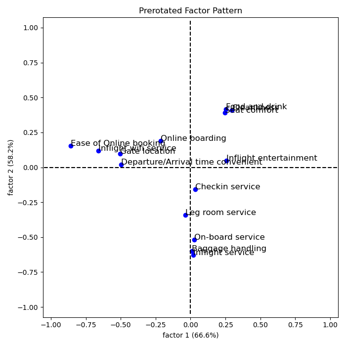
Unrotated loadings:

results.loadings

Out[123]: 
array([[ 0.41623784, -0.65850723,  0.12035065],
       [ 0.14214463, -0.4986264 ,  0.0204743 ],
       [ 0.30185314, -0.8578344 ,  0.15256493],
       [ 0.0965834 , -0.50311275,  0.09844108],
       [ 0.57728164,  0.25446329,  0.41662749],
       [ 0.46516202, -0.21285358,  0.19064456],
       [ 0.65348712,  0.24435365,  0.3914481 ],
       [ 0.84415447,  0.25585916,  0.04839901],
       [ 0.48650244,  0.02597749, -0.51911767],
       [ 0.36742193, -0.03771079, -0.34014596],
       [ 0.48111541,  0.01022714, -0.60139137],
       [ 0.27483868,  0.03324022, -0.15656155],
       [ 0.49262959,  0.0194701 , -0.62885468],
       [ 0.69879915,  0.29553957,  0.40822891]])

drawing drawing drawing

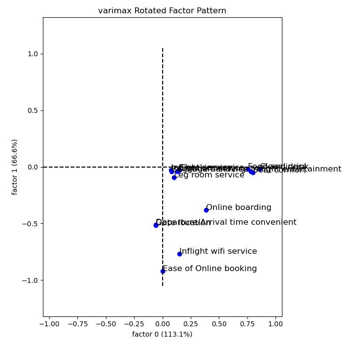
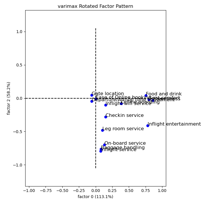
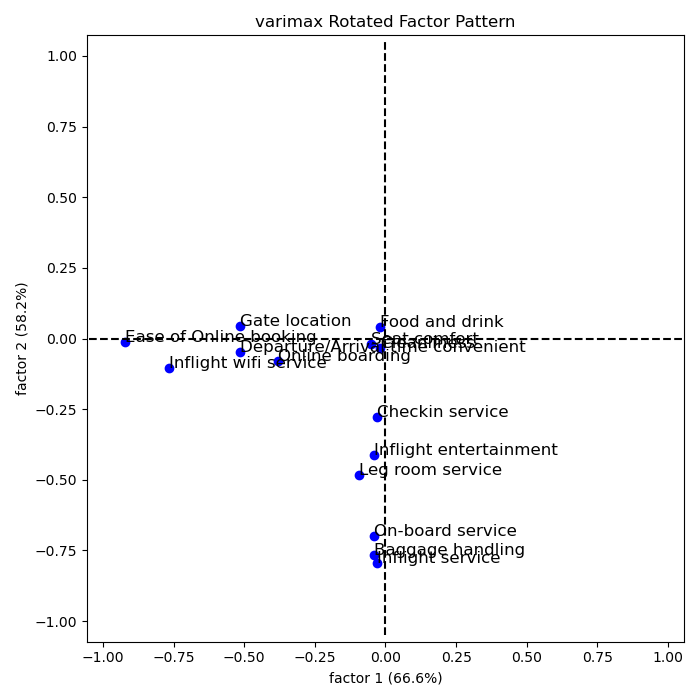
Rotated loadings:

results.rotate('varimax')
results.loadings

Out[132]: 
array([[ 0.14787756, -0.76735192, -0.10331135],
       [-0.05930589, -0.51341631, -0.04625023],
       [ 0.001848  , -0.92203905, -0.01057408],
       [-0.05756442, -0.51660793,  0.04409107],
       [ 0.75467628, -0.02013316,  0.04052768],
       [ 0.38346871, -0.38016993, -0.08031359],
       [ 0.79818003, -0.04952743, -0.02100997],
       [ 0.77983455, -0.04002052, -0.41310965],
       [ 0.13074484, -0.04093086, -0.69862226],
       [ 0.103968  , -0.09334843, -0.48228309],
       [ 0.07949962, -0.03954792, -0.76509083],
       [ 0.1492195 , -0.02964238, -0.27929841],
       [ 0.07811092, -0.02983718, -0.79468839],
       [ 0.86076469, -0.0192643 , -0.03205879]])

The higher a factor loading, the more important a variable is for said factor. Usually, a loading cutoff of 0.5 is used. This cutoff decides which variables belongs to which factor. Hence,

The first factor caontains variables 5, 7, 8, 14
The second factor contains variables 1, 2, 3, 4
The third factor contains variables 9, 11, 13

drawing drawing drawing

Recall that the 14 variables considered are:

['Inflight wifi service',
 'Departure/Arrival time convenient',
 'Ease of Online booking',
 'Gate location',
 'Food and drink',
 'Online boarding',
 'Seat comfort',
 'Inflight entertainment',
 'On-board service',
 'Leg room service',
 'Baggage handling',
 'Checkin service',
 'Inflight service',
 'Cleanliness']

Therefore, the three factors can be explained as:

Comfort: Food and Drink, Seat comfort, Inflight entertainment, Cleanliness
Convenience: In flight Wifi, Departure/Arrival time convenience, Online Booking, Gate Location.
Service: Onboard service, Baggage Handling, Inflight Service

Factor Scores

Factor scoring coefficient matrix:

results.factor_score_params()

Out[139]: 
array([[ 0.01729959, -0.24417132, -0.01322147],
       [-0.01900684, -0.08682621, -0.00894957],
       [-0.0535145 , -0.76064598,  0.05825796],
       [-0.0126019 , -0.0891501 ,  0.01693065],
       [ 0.22051131,  0.00780611,  0.10849854],
       [ 0.05676871, -0.06106693,  0.01001721],
       [ 0.26798272,  0.0022086 ,  0.10067651],
       [ 0.33992157,  0.02923623, -0.20999439],
       [-0.03919222,  0.00858151, -0.27956411],
       [-0.01631891, -0.00670421, -0.12531997],
       [-0.07114288,  0.01168981, -0.37920286],
       [ 0.00451548,  0.0009571 , -0.05573909],
       [-0.08440538,  0.01740522, -0.44418667],
       [ 0.403036  ,  0.02014393,  0.14256182]])

Factor scores:

results.factor_scoring()

Out[140]: 
array([[ 0.5894652 , -0.61037357, -1.52316734],
       [ 1.26600869,  0.46717871, -0.06557448],
       [-1.07729015,  0.62376949,  0.83407618],
       ...,
       [-1.3706222 ,  0.88601783, -0.62703381],
       [ 0.50028647, -0.14472913, -0.67078162],
       [-1.10915367,  0.18519492,  2.65380433]])

Principle Component Analysis

In factor analysis we model the observed variables as linear functions of the “factors.” In principal components, we create new variables that are linear combinations of the observed variables.

Notations and Model

Suppose we have a random vector $X=(X_1,X_2,...,X_p)^T$ with population variance matrix

$var(X) = \Sigma = [\sigma_1^2,\sigma_{12}^2,\cdots,\sigma_{1p}^2; \sigma_{21}^2,\sigma_{2}^2,\cdots,\sigma_{2p}^2; \cdots; \sigma_{p1}^2,\sigma_{p2}^2,\cdots,\sigma_p^2]$

Consider the linear combination

$Y_1 = e_{11}X_1 + e_{12}X_2 + \cdots + e_{1p}X_p$

$Y_2 = e_{21}X_1 + e_{22}X_2 + \cdots + e_{2p}X_p$

$\vdots$

$Y_p = e_{p1}X_1 + e_{p2}X_2 + \cdots + e_{pp}X_p$

Each of these can be considered as a multiple regression without intercepts.

For $Y_i, i=1,2,...,p$

$var(Y_i) = E[(Y_i-E(Y_i))^2] = E[(e_{11}(X_1-E(X_1))+ \cdots + e_{p1}(X_p-E(X_p)))^2] = {\displaystyle \sum_{k=1}^p\sum_{l=1}^pe_{ik}e_{il}\sigma_{kl} = e_i^T\Sigma e_i}$

and

$cov(Y_i,Y_j) = {\displaystyle \sum_{k=1}^p\sum_{l=1}^pe_{ik}e_{jl}\sigma_{kl} = e_i^T\Sigma e_j}$

PCA Procedure

First Principle Component (PCA1)

The first principal component is the linear combination of x-variables that has maximum variance (among all linear combinations). It accounts for as much variation in the data as possible.

We define the coefficeients for the first component in such as way that its variance is maximized, subject to the constraint that the sum of the squared coefficients is equal to 1. Namely, select $e_{11}, ..., e_{1p}$ to maximize

$var(Y_1) = e_1^T\Sigma e_1$

subject to

$e_1^Te_1 = {\displaystyle \sum_{j=1}^pe_{1j}^2 = 1}$

Second Principle Component (PCA2)

The second principal component is the linear combination of x-variables that accounts for as much of the remaining variation as possible, with the constraint that the correlation between the first and second component is 0.

Namely, select $e_{21}, ..., e_{2p}$ to maximize

$var(Y_2) = e_2^T\Sigma e_2$

subject to

$e_2^Te_2 = {\displaystyle \sum_{j=1}^pe_{2j}^2 = 1}$

and

$cov(Y_1,Y_2) = e_1^T\Sigma e_2 = 0$

i-th Principle Component (PCAi)

select $e_{i1}, ..., e_{ip}$ to maximize

$var(Y_2) = e_2^T\Sigma e_2$

subject to

$e_i^Te_i = {\displaystyle \sum_{j=1}^pe_{ij}^2 = 1}$

and

$cov(Y_1,Y_i) = e_1^T\Sigma e_i = 0$

$cov(Y_2,Y_i) = e_2^T\Sigma e_i = 0$

$\vdots$

$cov(Y_{i-1},Y_i) = e_{i-1}^T\Sigma e_i = 0$

Solution

Let $\lambda_1,...,\lambda_p$ denote the $p$ eigenvalues of $\Sigma$ with

$\lambda_1\geq \cdots \geq \lambda_p$

The $p$ corresponding eigenvectors are denoted as

$e_1,...,e_p$

It turns out that the elements for these eigenvectors are the coefficients of the principal components.

The variance for the $i\text{th}$ principle component is

$var(Y_i) = e_i^T\Sigma e_i = \lambda_i e_i^Te_i = \lambda_i$

and

$cov(Y_i,Y_j) = e_i^T\Sigma e_j = 0$

By spectral decomposition theorem, we have

$\Sigma = {\displaystyle \sum_{i=1}^p\lambda_ie_ie_i^T}$

The idea behind PCA is to approximate the covariance matrix by tahe first $k$ components, namely

$\Sigma \approx {\displaystyle \sum_{i=1}^k\lambda_ie_ie_i^T}$

To understand this, we define the total variation of $X$ as the trace of the covariance matrix, which is the sum of the variances of the individual variables. That is

$\text{trace}(\Sigma) = \sigma_1^2 + \sigma_2^2 + \cdots + \sigma_p^2 = \lambda_1 + \lambda_2 + \cdots + \lambda_p$

Thus, the $i\text{th}$ principle component explains the following proportion of the total variation:

$\dfrac{\lambda_i}{\lambda_1 + \lambda_2 + \cdots + \lambda_p}$

Therefore, the first $k$ principle component would explain the following proportion of the total variation:

$\dfrac{\lambda_1+ \lambda_2 + \cdots + \lambda_k}{\lambda_1 + \lambda_2 + \cdots + \lambda_p}$

Example

We use the same data as the example in factor analysis and still use the statsmodels to realize PCA algorithm.

class statsmodels.multivariate.pca.PCA(data, ncomp=None, standardize=True, demean=True, normalize=True, gls=False, weights=None, method='svd', missing=None, tol=5e-08, max_iter=1000, tol_em=5e-08, max_em_iter=100, svd_full_matrices=False)

Parameters:
  data: array_like
    Variables in columns, observations in rows.

  ncomp: int, optional
    Number of components to return. If None, returns the as many as the smaller of the number of rows or columns in data.

Data Analysis

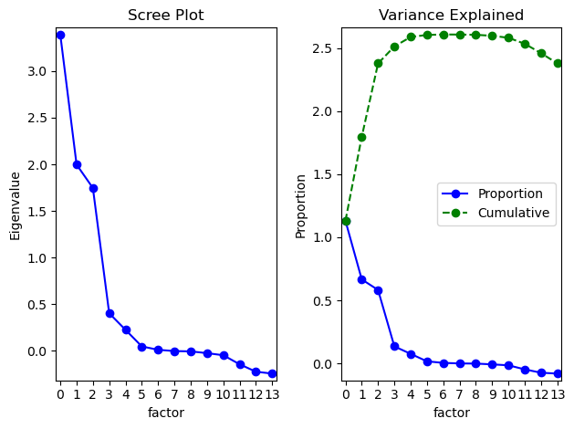
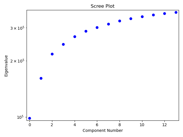
First, let examine the eigenvalues to determine how many principle components should be considered.

results = sm.PCA(x, method = 'nipals')

Eigenvalues:

results.eigenvals

Out[292]: 
   98351.323505
   62565.929983
   56669.672061
   27624.149068
   24520.057939
   17897.417218
   13734.114836
   13188.024211
   12018.743569
    9481.617208
   8586.135543
   7465.813471
   6741.359084
   4819.642304
Name: eigenvals, dtype: float64

Below is the cumulative percentage obtained by adding the successive proportions of variation explained by each eigenvalue.

[0.2704455857730838,
4424888179407722,
5983185730459308,
674279209974658,
7417042450053434,
7909184020783133,
8286843476664585,
8649486581584533,
8979976912454709,
9240701570614314,
9476802354388428,
9682096622480078,
9867469908923509,
0]

And below is the scree plot of the eigenvalues, to cover 80% of the variation, we need 7 principle components.

drawing

PCA

Next, we compute the principal component scores using loadings.

results = sm.PCA(x,7,method = 'nipals')

Loadings: ncomp by nvar array of principal component loadings for constructing the factors

results.loadings

Out[316]: 
                                     comp_0    comp_1  ...    comp_5    comp_6
Inflight wifi service              0.229428  0.448378  ... -0.095192 -0.222513
Departure/Arrival time convenient  0.089759  0.423246  ... -0.007206  0.600277
Ease of Online booking             0.158174  0.530357  ... -0.022008 -0.133023
Gate location                      0.059700  0.430829  ...  0.175737 -0.304796
Food and drink                     0.307710 -0.170796  ...  0.004112 -0.168312
Online boarding                    0.277880  0.157983  ... -0.185668  0.199786
Seat comfort                       0.345547 -0.159879  ...  0.066538  0.194946
Inflight entertainment             0.431140 -0.174646  ... -0.058597 -0.034484
On-board service                   0.277950 -0.050805  ... -0.225194  0.414931
Leg room service                   0.226631  0.001451  ...  0.840270  0.153394
Baggage handling                   0.268328 -0.040025  ... -0.206501 -0.242053
Checkin service                    0.178831 -0.044026  ...  0.238955 -0.294801
Inflight service                   0.270867 -0.046380  ... -0.240973 -0.175362
Cleanliness                        0.357168 -0.185636  ...  0.050917 -0.013267

[14 rows x 7 columns]

For PCA, loadings are the same as eigenvectors:

results.eigenvecs

Out[319]: 
    eigenvec_0  eigenvec_1  eigenvec_2  ...  eigenvec_4  eigenvec_5  eigenvec_6
   0.229428    0.448378   -0.069026  ...   -0.226457   -0.095192   -0.222513
   0.089759    0.423246    0.007340  ...    0.407065   -0.007206    0.600277
   0.158174    0.530357   -0.069181  ...   -0.158245   -0.022008   -0.133023
   0.059700    0.430829   -0.060077  ...    0.152772    0.175737   -0.304796
   0.307710   -0.170796   -0.345555  ...   -0.000059    0.004112   -0.168312
   0.277880    0.157983   -0.169104  ...   -0.095087   -0.185668    0.199786
   0.345547   -0.159879   -0.315762  ...    0.102873    0.066538    0.194946
   0.431140   -0.174646   -0.070707  ...   -0.145801   -0.058597   -0.034484
   0.277950   -0.050805    0.386667  ...   -0.003841   -0.225194    0.414931
   0.226631    0.001451    0.299764  ...   -0.322904    0.840270    0.153394
  0.268328   -0.040025    0.429205  ...   -0.005617   -0.206501   -0.242053
  0.178831   -0.044026    0.144506  ...    0.764468    0.238955   -0.294801
  0.270867   -0.046380    0.437012  ...   -0.004266   -0.240973   -0.175362
  0.357168   -0.185636   -0.314051  ...    0.070783    0.050917   -0.013267

[14 rows x 7 columns]

Scores (factors):

results.scores

Out[320]: 
         comp_0    comp_1    comp_2    comp_3    comp_4    comp_5    comp_6
0      0.008190  0.004232  0.004682 -0.005359 -0.009091 -0.001165  0.002354
1      0.004861 -0.009642 -0.002719  0.003397 -0.004955 -0.000080  0.001975
2     -0.009640 -0.001508 -0.000549 -0.001721 -0.004047 -0.008081 -0.007137
3     -0.011144 -0.010268 -0.013178  0.007958  0.003495  0.000297 -0.000113
4     -0.006631  0.001024 -0.006514 -0.002883  0.006178  0.003718 -0.007019
        ...       ...       ...       ...       ...       ...       ...
25971  0.002635 -0.003803 -0.000637  0.002205  0.002847 -0.009210 -0.003536
25972  0.008337  0.004220  0.003988  0.000708  0.003685  0.005225 -0.005247
25973 -0.004935  0.002529  0.008071 -0.008449  0.014689  0.003291 -0.001168
25974  0.004313 -0.000786 -0.000022 -0.000034  0.003890 -0.009497 -0.008091
25975 -0.013136  0.006459 -0.009547 -0.009968  0.000275  0.004297  0.005153

[25976 rows x 7 columns]

Interpretation

To interpret each component, we should compute the correlations between the original data and each principle component.

x_np = x.to_numpy()
y_np = results.factors.to_numpy()
corrM = np.corrcoef(np.transpose(x_np),np.transpose(y_np))
corrP = corrM[:14,14:]

Results:

               PCA1          PCA2         PCA3         PCA4         PCA5         PCA6         PCA7
X1   array([[4.4643e-01,  6.9587e-01, -1.0195e-01,  1.9242e-01, -2.2002e-01, -7.9015e-02, -1.6180e-01],
X2         [ 1.7466e-01,  6.5686e-01,  1.0842e-02, -3.1111e-01,  3.9549e-01, -5.9812e-03,  4.3648e-01],
X3         [ 3.0778e-01,  8.2310e-01, -1.0218e-01,  1.2615e-01, -1.5375e-01, -1.8268e-02, -9.6726e-02],
X4         [ 1.1616e-01,  6.6863e-01, -8.8735e-02, -4.7870e-01,  1.4843e-01,  1.4587e-01, -2.2163e-01],
X5         [ 5.9875e-01, -2.6507e-01, -5.1040e-01, -2.1042e-01, -5.7728e-05,  3.4130e-03, -1.2239e-01],
X6         [ 5.4071e-01,  2.4519e-01, -2.4977e-01,  6.1012e-01, -9.2383e-02, -1.5412e-01,  1.4527e-01],
X7         [ 6.7237e-01, -2.4813e-01, -4.6639e-01,  1.0980e-02,  9.9949e-02,  5.5231e-02,  1.4175e-01],
X8         [ 8.3892e-01, -2.7105e-01, -1.0444e-01, -2.2680e-01, -1.4166e-01, -4.8639e-02, -2.5074e-02],
X9         [ 5.4084e-01, -7.8848e-02,  5.7112e-01, -9.8156e-03, -3.7317e-03, -1.8692e-01,  3.0171e-01],
X10        [ 4.4098e-01,  2.2526e-03,  4.4276e-01,  6.6841e-02, -3.1372e-01,  6.9747e-01,  1.1154e-01],
X11        [ 5.2212e-01, -6.2117e-02,  6.3395e-01, -1.0243e-01, -5.4570e-03, -1.7141e-01, -1.7600e-01],
X12        [ 3.4797e-01, -6.8327e-02,  2.1344e-01,  4.1332e-01,  7.4273e-01,  1.9835e-01, -2.1436e-01],
X13        [ 5.2706e-01, -7.1981e-02,  6.4548e-01, -1.2812e-01, -4.1446e-03, -2.0002e-01, -1.2751e-01],
X14        [ 6.9499e-01, -2.8810e-01, -4.6386e-01, -1.1913e-01,  6.8771e-02,  4.2264e-02, -9.6470e-03]])

Similar to factor analysis, if the correlation is greater than 0.5, we consider it as important. Thus,

PCA1: +X5, +X6, +X7, +X8, +X9, +X11, +X13, +X14
PCA2: +X1, +X2, +X3, +X4
PCA3: -X5, +X9, +X11, +X13
PCA4: +X6
PCA5: +X12
PCA6: +X10
PCA7: +X2

We can also check that the covariance matrix of the principle components is an identical matrix.

corrM[14:,14:]

Out[337]: 
array([[ 1.0000e+00, -4.6926e-08, -2.1001e-11,  5.2909e-17, -1.0799e-16,  3.2309e-16, -2.3419e-17],
       [-4.6926e-08,  1.0000e+00,  4.7947e-08, -3.0626e-15, -3.4868e-16, -6.9389e-17,  2.2183e-16],
       [-2.1001e-11,  4.7947e-08,  1.0000e+00, -3.2156e-08, -3.6600e-09, -6.1573e-13,  1.2863e-15],
       [ 5.2909e-17, -3.0626e-15, -3.2156e-08,  1.0000e+00, -4.7749e-08,  6.5655e-15, -2.2985e-17],
       [-1.0799e-16, -3.4868e-16, -3.6600e-09, -4.7749e-08,  1.0000e+00, -3.7023e-08,  3.4079e-13],
       [ 3.2309e-16, -6.9389e-17, -6.1573e-13,  6.5655e-15, -3.7023e-08,  1.0000e+00, -3.9001e-08],
       [-2.3419e-17,  2.2183e-16,  1.2863e-15, -2.2985e-17,  3.4079e-13, -3.9001e-08,  1.0000e+00]])

One can interpret these component by component. One method of deciding how many components to include is to choose only those that give unambiguous results, i.e., where no variable appears in two different columns as a significant contribution.

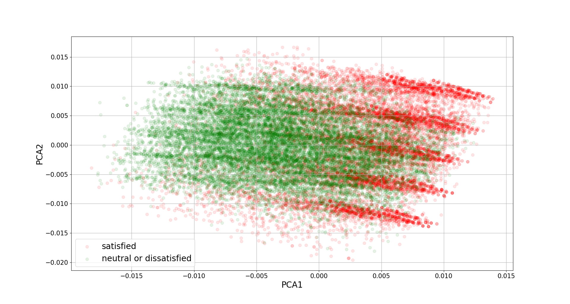
To complete the analysis we often would like to produce a scatter plot of the component scores. For example, below is a figure plotting the second component against the first one, where red dots represent satisfied and green dots represent neutral or unsatisfied.

finalDF = pd.concat([results.scores, data[['satisfaction']]], axis = 1)

fig = plt.figure()
ax = fig.add_subplot(1,1,1) 
ax.set_xlabel('PCA1', fontsize = 15)
ax.set_ylabel('PCA2', fontsize = 15)
targets = ['satisfied', 'neutral or dissatisfied']
colors = ['r', 'g']
for target, color in zip(targets,colors):
    indicesToKeep = finalDF['satisfaction'] == target
    ax.scatter(finalDF.loc[indicesToKeep, 'comp_0']
               , finalDF.loc[indicesToKeep, 'comp_1']
               , c = color
               , s = 50, alpha = 0.1)
ax.legend(targets)
ax.grid()

drawing

For more examples, here is an example using sklearn and the Iris dataset.

Twitter Facebook LinkedIn

Chao Huang

Statistics [29]: Factor and Principle Component Analysis

Factor Analysis

Notations

Assumptions

Mean

Variance

Correlation

Model Properties

Principle Component Method

Maximum Likelihood Estimation Method

Goodness of Fit

Factor Rotations

Varimax Rotation

Estimation of Factor Scores

Ordinary Least Squares (OLS)

Weightead Least Squares (WLS)

Example

Data

Factor Analysis

Factor Scores

Principle Component Analysis

Notations and Model

PCA Procedure

First Principle Component (PCA1)

Second Principle Component (PCA2)

i-th Principle Component (PCAi)

Solution

Example

Data Analysis

PCA

Interpretation

Table of Contents

Comments