Statistics [30]: Clustering Analysis

5 minute read

Published: January 30, 2021

Clustering analysis is the task of grouping a set of objects in such a way that objects in the same group are more similar to each other than to those in other groups.

Measurement of Association

Metrics

Minkowski Distance

$d(\textbf{X}_i,\textbf{X}_j) = {\displaystyle \left[\sum_{k=1}^p\left|X_{ik}-X_{jk}\right|^m\right]^{1\text{/}m}}$

When $m=1$ , it is Absolute Distance

$d(\textbf{X}_i,\textbf{X}_j) = {\displaystyle \sum_{k=1}^p\left|X_{ik}-X_{jk}\right|}$

When $m=2$ , it is Euclidean Distance

$d(\textbf{X}_i,\textbf{X}_j) = {\displaystyle \sqrt{\sum_{i=k}^p(X_{ik}-X_{jk})^2}}$

When $m=\infty$ , it is Chebysheve Distance

$d(\textbf{X}_i,\textbf{X}_j) = {\displaystyle \max_{1\leq k\leq p}\left|X_{ik}-X_{jk}\right|}$

Standardized Euclidean Distance

Let the covariance matrix of $X$ be $S$ , which is

$S = {\displaystyle \dfrac{1}{n-1}\sum_{i=1}^{n}(\textbf{X}_i-\bar{\textbf{X}})(\textbf{X}_i-\bar{\textbf{X}})^T}$

Standardized Euclidean distance:

$d(\textbf{X}_i,\textbf{X}_j) = {\displaystyle \sqrt{\sum_{i=k}^p\dfrac{(X_{ik}-X_{jk})^2}{S_{ll}}}}$

Mahalanobis Distance

$d(\textbf{X}_i,\textbf{X}_j) = {\displaystyle \left[ (\textbf{X}_i-\textbf{X}_j)^TS^{-1}(\textbf{X}_i-\textbf{X}_j) \right]^{1\text{/}2}}$

If $\textbf{X}_i,\textbf{X}_j$ are independent, namely, the covariance matrix $S$ is a diagonal matrix, then Mahalanobis distance becomes standardized Euclidean distance.

Canberra Metric

$d(\textbf{X}_i,\textbf{X}_j) = {\displaystyle \sum_{k=1}^p\dfrac{|X_{ik}-X_{jk}|}{X_{ik}+ X_{jk}}}$

Czekanowski Coefficient

$d(\textbf{X}_i,\textbf{X}_j) = 1 - {\displaystyle \dfrac{2\sum_{k=1}^p\min(X_{ik},X_{jk})}{\sum_{k=1}^p(X_{ik}+ X_{jk})} = \dfrac{\sum_{k=1}^p\left[\max(X_{ik},X_{jk})-\min(X_{ik},X_{jk})\right]}{\sum_{k=1}^p(X_{ik}+ X_{jk})}}$

Properties of Metrics

Symmetry: $d(\textbf{X}_i,\textbf{X}_j) = d(\textbf{X}_j,\textbf{X}_i)$
Positivity: $d(\textbf{X}_i,\textbf{X}_j)>0,\ \ \textbf{X}_i\neq \textbf{X}_j$
Identity: $d(\textbf{X}_i,\textbf{X}_j)=0,\ \ \textbf{X}_i= \textbf{X}_j$
Triangle Inequality: $d(\textbf{X}_i,\textbf{X}_k)\leq d(\textbf{X}_i,\textbf{X}_j) + d(\textbf{X}_j,\textbf{X}_k)$

Agglomerative Clustering

Basic Ideas

In agglomerative hierarchical algorithms, we start by defining each data point as a cluster. Then, the two closest clusters are combined into a new cluster. In each subsequent step, two existing clusters are merged into a single cluster.

There are several methods for measuering association between the clusters:

Single Linkage: $d_{12} = \min_{i\text{,}j}d(\textbf{X}_i,\textbf{X}_j)$
Complete Linkage: $d_{12} = \max_{i\text{,}j}d(\textbf{X}_i,\textbf{X}_j)$
Average Linkage: $d_{12} = \dfrac{1}{kl}{\displaystyle \sum_{i=1}^k\sum_{j=1}^ld(\textbf{X}_i,\textbf{X}_j)}$
Centroid Method: $d_{12} = d(bar{X},\bar{Y})$
Ward’s Method: ANOVA based approach

Example

Below is an example using package sklearn and the Iris dataset.

class sklearn.cluster.AgglomerativeClustering(n_clusters=2, *, affinity='euclidean', memory=None, connectivity=None, compute_full_tree='auto', linkage='ward', distance_threshold=None, compute_distances=False)

Data

import pandas as pd
import numpy as np
import matplotlib.pyplot as plt
from sklearn.preprocessing import normalize
from sklearn.cluster import AgglomerativeClustering
from sklearn.datasets import load_iris

# load data
iris = load_iris()
data = iris.data
data[:5]

# normalize data
data_scaled = normalize(data)
data_scaled = pd.DataFrame(data_scaled, columns=['sepalL','sepalW','petalL','petalW'])
data_scaled.head()

# Before normalization
array([[5.1, 3.5, 1.4, 0.2],
       [4.9, 3. , 1.4, 0.2],
       [4.7, 3.2, 1.3, 0.2],
       [4.6, 3.1, 1.5, 0.2],
       [5. , 3.6, 1.4, 0.2]])

# After nromalization
     sepalL    sepalW    petalL    petalW
0  0.803773  0.551609  0.220644  0.031521
1  0.828133  0.507020  0.236609  0.033801
2  0.805333  0.548312  0.222752  0.034269
3  0.800030  0.539151  0.260879  0.034784
4  0.790965  0.569495  0.221470  0.031639

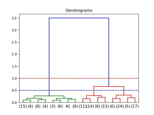
Draw the dendrogram to help us decide the number of clusters:

from scipy.cluster.hierarchy import dendrogram,linkage
plt.figure()  
plt.title("Dendrograms")  
dend = dendrogram(linkage(data_scaled, method='ward'))

drawing

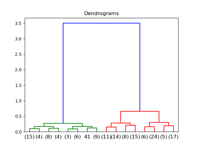
The x-axis contains the samples and y-axis represents the distance between these samples. If the threshold is 1.0, there will be two clusters; if the threshold is 0.5, there will be 3 clusters.

drawing

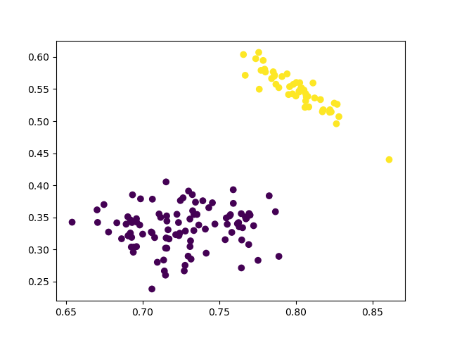
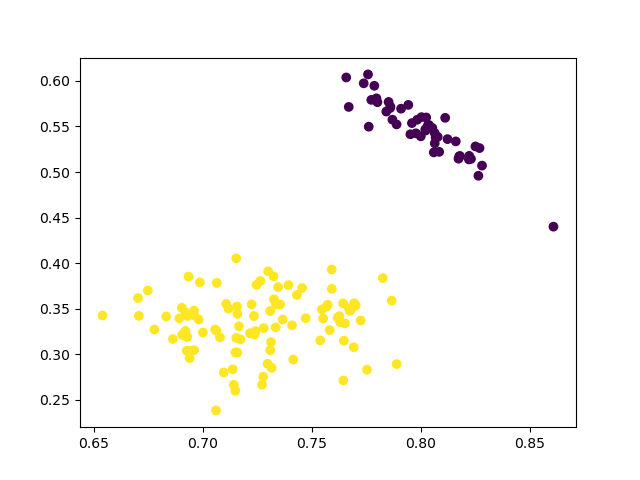
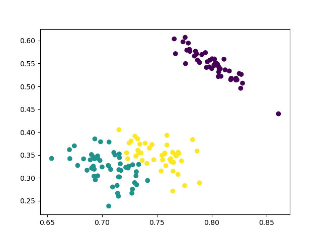
2 Clusters

First, let’s see the results of two clusters.

cluster = AgglomerativeClustering(n_clusters=2, affinity='euclidean', linkage='ward')  
cluster.fit_predict(data_scaled)

array([1, 1, 1, 1, 1, 1, 1, 1, 1, 1, 1, 1, 1, 1, 1, 1, 1, 1, 1, 1, 1, 1,
       1, 1, 1, 1, 1, 1, 1, 1, 1, 1, 1, 1, 1, 1, 1, 1, 1, 1, 1, 1, 1, 1,
       1, 1, 1, 1, 1, 1, 0, 0, 0, 0, 0, 0, 0, 0, 0, 0, 0, 0, 0, 0, 0, 0,
       0, 0, 0, 0, 0, 0, 0, 0, 0, 0, 0, 0, 0, 0, 0, 0, 0, 0, 0, 0, 0, 0,
       0, 0, 0, 0, 0, 0, 0, 0, 0, 0, 0, 0, 0, 0, 0, 0, 0, 0, 0, 0, 0, 0,
       0, 0, 0, 0, 0, 0, 0, 0, 0, 0, 0, 0, 0, 0, 0, 0, 0, 0, 0, 0, 0, 0,
       0, 0, 0, 0, 0, 0, 0, 0, 0, 0, 0, 0, 0, 0, 0, 0, 0, 0], dtype=int64)

Visualization:

plt.figure()  
plt.scatter(data_scaled['sepalL'], data_scaled['sepalW'], c=cluster.labels_) 

drawing

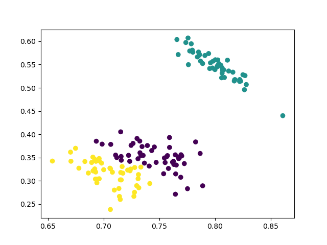
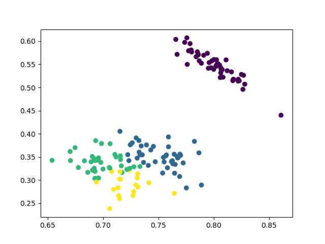
3 Clusters

cluster = AgglomerativeClustering(n_clusters=3, affinity='euclidean', linkage='ward')  
cluster.labels_

array([1, 1, 1, 1, 1, 1, 1, 1, 1, 1, 1, 1, 1, 1, 1, 1, 1, 1, 1, 1, 1, 1,
       1, 1, 1, 1, 1, 1, 1, 1, 1, 1, 1, 1, 1, 1, 1, 1, 1, 1, 1, 1, 1, 1,
       1, 1, 1, 1, 1, 1, 0, 0, 0, 0, 0, 0, 0, 0, 0, 0, 0, 0, 0, 0, 0, 0,
       0, 0, 0, 0, 0, 0, 2, 0, 0, 0, 0, 0, 0, 0, 0, 0, 0, 2, 0, 0, 0, 0,
       0, 0, 0, 0, 0, 0, 0, 0, 0, 0, 0, 0, 2, 2, 2, 2, 2, 2, 2, 2, 2, 2,
       0, 2, 2, 2, 2, 2, 2, 2, 2, 2, 2, 2, 2, 2, 2, 2, 2, 0, 2, 2, 2, 0,
       2, 2, 2, 2, 2, 2, 0, 2, 2, 2, 2, 2, 2, 2, 2, 2, 2, 2], dtype=int64)

Visualization:

plt.figure()  
plt.scatter(data_scaled['sepalL'], data_scaled['sepalW'], c=cluster.labels_) 

drawing

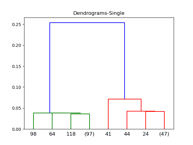
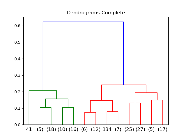
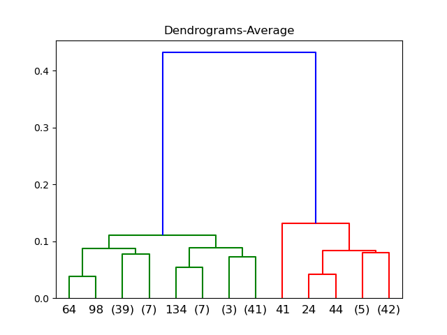
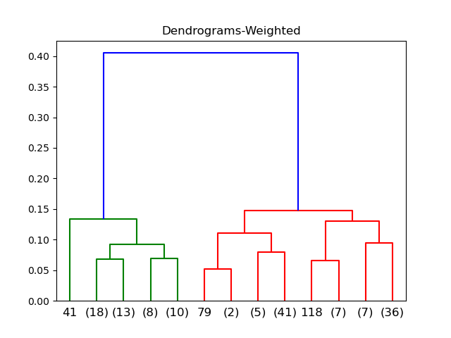
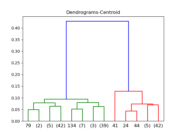
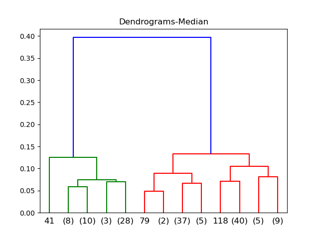
Comparison of Different Linkage Methods

Single

drawing

Complete

drawing

Average

drawing

Weighted

drawing

Centroid

drawing

Median

drawing

Ward

drawing

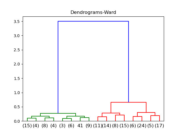
ANOVA

After obtaining the clusters, ANOVA test can be done for each of the plants, comparing the means across clusters. If the $p$ value is small, we may conclude that there are significant differences across clusters.

K-Means CLustering

Procedures

Partition the items into $K$ initial clusters.
Loop thorugh the items and assign each item to the cluster whose center is closest. (Accordingly, the centroids of the clusters receiving and losing the item should be recalculated.)
Repeat 2 until no more assignments.

Example

We repeat the above example using the Iris dataset.

from sklearn.cluster import KMeans

kmeans2 = KMeans(n_clusters=2, random_state=0).fit(data_scaled)
kmeans3 = KMeans(n_clusters=3, random_state=0).fit(data_scaled)
kmeans4 = KMeans(n_clusters=4, random_state=0).fit(data_scaled)


plt.figure()  
plt.scatter(data_scaled['sepalL'], data_scaled['sepalW'], c=kmeans2.labels_) 

plt.figure()  
plt.scatter(data_scaled['sepalL'], data_scaled['sepalW'], c=kmeans3.labels_) 

plt.figure()  
plt.scatter(data_scaled['sepalL'], data_scaled['sepalW'], c=kmeans4.labels_) 

2 clusters

drawing

3 clusters

drawing

4 clusters

drawing

The results are similiar to the agglomerative clustering and we can also run ANOVA test to compare the means of diffearent clusters.

Twitter Facebook LinkedIn

Chao Huang

Statistics [30]: Clustering Analysis

Measurement of Association

Metrics

Minkowski Distance

Standardized Euclidean Distance

Mahalanobis Distance

Canberra Metric

Czekanowski Coefficient

Properties of Metrics

Agglomerative Clustering

Basic Ideas

Example

Data

2 Clusters

3 Clusters

Comparison of Different Linkage Methods

ANOVA

K-Means CLustering

Procedures

Example

Table of Contents

Comments