
Data Modeling [02]: Scikit-Learn
Published:
Scikit-Learn contains a broad selection of standard supervised and unsupervised machine learning methods with tools for model selection and evaluation, data transformation, data loading, and model persistence. These models can be used for classification, clustering, regression, dimensionality reduction, and other common tasks. Let’s learn the basic of scikit-learnin dealing with classification and regression problems through several simple examples. Clustering and dimensionality examples can be referenced to Clustering Analysis and Factor and Principle Component Analysis respectively.
Classification
Data Loading and Inspection
Load the Kaggle titannic dataset into workspace:
import pandas as pd
import numpy as np

train = pd.read_csv('titanic/train.csv')
test = pd.read_csv('titanic/test.csv')
Check whether there are null values in the dataset:
train.info()
<class 'pandas.core.frame.DataFrame'>
RangeIndex: 891 entries, 0 to 890
Data columns (total 12 columns):
 #   Column       Non-Null Count  Dtype
---  ------       --------------  -----
 0   PassengerId  891 non-null    int64
 1   Survived     891 non-null    int64
 2   Pclass       891 non-null    int64
 3   Name         891 non-null    object
 4   Sex          891 non-null    object
 5   Age          714 non-null    float64
 6   SibSp        891 non-null    int64
 7   Parch        891 non-null    int64
 8   Ticket       891 non-null    object
 9   Fare         891 non-null    float64
 10  Cabin        204 non-null    object
 11  Embarked     889 non-null    object
dtypes: float64(2), int64(5), object(5)
memory usage: 83.7+ KB
Data Cleaning and Preparation
The typical task is to predict whether a passenger would survive based on features in the data. Here, we use ‘Pclass’, ‘Sex’ and ‘Age’ as predictors to predict the survival status ‘Sirvoved’. As ‘Age’ has null values, we should first fill those values.
train['Age'] = train['Age'].fillna(train['Age'].median())
test['Age'] = train['Age'].fillna(test['Age'].median())
As ‘Sex’ column is not numeric, we should add an encoded version of the Sex column:
train['IsFemale'] = (train['Sex'] == 'female').astype(int)
test['IsFemale'] = (test['Sex'] == 'female').astype(int)
Hence,
X_train = train[['Pclass', 'Age', 'IsFemal']].values
X_test  = test[['Pclass', 'Age', 'IsFemal']].values
y_train = train[['Survived']].values
Model Building and Prediction
We use the logistic model for prediction.
from sklearn.linear_model import LogisticRegression
model = LogisticRegression().fit(X_train, y_train)
y_predict = model.predict(X_test)

y_predict
Out[181]:
array([0, 0, 0, 0, 1, 0, 0, 0, 1, 0, 0, 0, 1, 0, 1, 1, 0, 0, 1, 1, 0, 0,
       1, 1, 1, 0, 1, 0, 1, 0, 0, 0, 1, 0, 1, 0, 1, 1, 0, 0, 0, 1, 0, 1,
       1, 0, 1, 0, 1, 1, 1, 0, 1, 1, 0, 0, 0, 0, 0, 1, 0, 0, 0, 1, 1, 1,
       1, 1, 1, 1, 1, 0, 1, 1, 1, 1, 0, 1, 0, 1, 0, 0, 1, 0, 0, 0, 1, 1,
       1, 0, 1, 0, 1, 0, 0, 0, 1, 0, 1, 0, 1, 0, 0, 0, 0, 0, 0, 0, 0, 0,
       0, 1, 1, 1, 1, 0, 0, 1, 1, 1, 1, 0, 1, 0, 0, 1, 0, 1, 0, 0, 0, 1,
       0, 0, 0, 0, 0, 0, 1, 0, 1, 1, 1, 0, 1, 0, 1, 0, 0, 0, 1, 0, 0, 0,
       0, 0, 1, 1, 1, 1, 0, 0, 1, 0, 0, 1, 1, 0, 1, 1, 0, 0, 0, 0, 0, 1,
       1, 0, 1, 1, 0, 1, 1, 0, 1, 0, 1, 0, 0, 0, 0, 1, 0, 0, 0, 0, 1, 0,
       0, 1, 1, 0, 0, 1, 0, 1, 1, 0, 1, 0, 0, 0, 0, 1, 1, 0, 1, 0, 1, 0,
       1, 0, 1, 0, 1, 1, 0, 1, 0, 0, 0, 1, 0, 0, 1, 0, 0, 0, 1, 1, 1, 1,
       0, 0, 0, 0, 1, 0, 1, 0, 1, 0, 0, 0, 0, 0, 0, 0, 1, 0, 0, 0, 1, 0,
       0, 0, 1, 0, 0, 0, 1, 0, 1, 0, 0, 1, 0, 0, 0, 0, 0, 0, 1, 1, 1, 0,
       0, 1, 0, 0, 1, 1, 0, 1, 0, 0, 1, 0, 1, 0, 0, 0, 0, 0, 1, 1, 1, 0,
       0, 1, 0, 0, 0, 1, 1, 1, 1, 0, 0, 0, 0, 0, 0, 1, 1, 0, 1, 0, 0, 0,
       1, 0, 0, 1, 0, 1, 0, 0, 0, 0, 0, 0, 0, 1, 0, 1, 0, 1, 0, 1, 1, 0,
       0, 0, 1, 1, 1, 0, 0, 1, 0, 1, 1, 0, 1, 1, 0, 1, 1, 0, 0, 1, 1, 0,
       1, 1, 1, 0, 1, 0, 0, 0, 1, 1, 0, 1, 0, 0, 0, 0, 0, 1, 0, 0, 0, 1,
       0, 1, 0, 0, 1, 0, 1, 1, 1, 0, 0, 1, 1, 1, 1, 1, 1, 0, 1, 0, 0, 0],
      dtype=int64)
Cross-Validation
Logistic regression has estimator class with built-in cross-validation:
from sklearn.linear_model import LogisticRegressionCV
model_cv = LogisticRegressionCV(cv = 10)  # Stratified 10-Folds cross-validation
model_cv.fit(X_train, y_train)
model_cv.scores is a dict with classes as the keys, and the values as the grid of scores obtained during cross-validating each fold, after doing an OvR (One-vs-Rest) for the corresponding class. Each dict value has shape (n_folds, n_cs), where Cs describes the inverse of regularization strength. If Cs is as an int, then a grid of Cs values are chosen in a logarithmic scale between 1e-4 and 1e4. Cs is 10 by default.
model_cv.scores_
Out[203]:
{1: array([[0.61111111, 0.61111111, 0.7       , 0.71111111, 0.78888889,
            0.78888889, 0.78888889, 0.78888889, 0.78888889, 0.78888889],
           [0.61797753, 0.61797753, 0.6741573 , 0.73033708, 0.78651685,
            0.79775281, 0.79775281, 0.79775281, 0.79775281, 0.79775281],
           [0.61797753, 0.61797753, 0.69662921, 0.74157303, 0.73033708,
            0.74157303, 0.74157303, 0.74157303, 0.74157303, 0.74157303],
           [0.61797753, 0.61797753, 0.80898876, 0.80898876, 0.83146067,
            0.83146067, 0.83146067, 0.83146067, 0.83146067, 0.83146067],
           [0.61797753, 0.61797753, 0.74157303, 0.78651685, 0.80898876,
            0.80898876, 0.80898876, 0.80898876, 0.80898876, 0.80898876],
           [0.61797753, 0.61797753, 0.70786517, 0.80898876, 0.78651685,
            0.78651685, 0.78651685, 0.78651685, 0.78651685, 0.78651685],
           [0.61797753, 0.61797753, 0.76404494, 0.80898876, 0.7752809 ,
            0.78651685, 0.78651685, 0.78651685, 0.78651685, 0.78651685],
           [0.61797753, 0.61797753, 0.74157303, 0.75280899, 0.76404494,
            0.76404494, 0.76404494, 0.76404494, 0.76404494, 0.76404494],
           [0.61797753, 0.61797753, 0.73033708, 0.85393258, 0.82022472,
            0.82022472, 0.82022472, 0.82022472, 0.82022472, 0.82022472],
           [0.60674157, 0.60674157, 0.73033708, 0.79775281, 0.79775281,
            0.79775281, 0.79775281, 0.79775281, 0.79775281, 0.79775281]])}

model.scores_[1].shape
Out[209]: (10, 10)
Regression
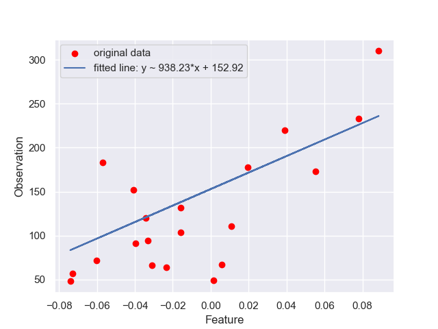
Ordinary Least Squares
For this example, let’s use the diabetes dataset.
from sklearn import datasets, linear_model
X, y = datasets.load_diabetes(return_X_y=True)

# choose the second feature for regression
X_ = X[:, np.newaxis, 2]

# split the data into training and testing sets
X_train = X_[:-20]
X_test = X_[-20:]
y_train = y[:-20]
y_test = y[-20:]

# train the model
model = linear_model.LinearRegression().fit(X_train, y_train)

# prediction
y_pred = model.predict(X_test) # model.coef_[0]*X_test + model.intercept_

# evaluation
r2_score(y_test, y_pred)
Out[242]: 0.47257544798227147

mean_squared_error(y_test, y_pred)
Out[243]: 2548.0723987259694

# plotting
plt.figure()
plt.scatter(X_test, y_test, label='original data', color = 'red')
plt.plot(X_test, y_pred, label = 'fitted line: y ~ 938.23*x + 152.92')
plt.xlabel('Feature')
plt.ylabel('Observation')
plt.legend()
plt.show()
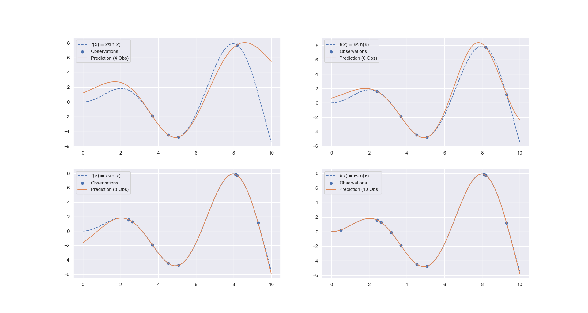
Gaussian Process Regression
For this example, let’s try to fit the function y = x*sin(x).
X = np.linspace(0,10,1000).reshape(-1, 1)
y = X * np.sin(X)
For training the model, first choose a few samples:
rng = np.random.RandomState(1)
training_indices = rng.choice(np.arange(y.size), size=6, replace=False)  # sample size is 6
X_train, y_train = X[training_indices], y[training_indices]
Train the model using a RBF kernel
from sklearn.gaussian_process import GaussianProcessRegressor
from sklearn.gaussian_process.kernels import RBF

kernel = 1 * RBF(length_scale=1.0, length_scale_bounds=(1e-2, 1e2))
gaussian_process = GaussianProcessRegressor(kernel=kernel, n_restarts_optimizer=9)
model = gaussian_process.fit(X_train, y_train)
Plot the results with different number of training samples:
y_pred = gaussian_process.predict(X)

fig, axes = plt.subplots(2,2)
axes[0,0].plot(X, y, label=r"$f(x) = x \sin(x)$", linestyle="--")
axes[0,0].scatter(X_train, y_train, label="Observations")
axes[0,0].plot(X, y_pred, label="Prediction (4 Obs)")
axes[0,0].legend()

# the other three are plotted similarly
Comments