
Data Modeling [03]: Pytorch
Published:
For non-deep-learning models, scikit-learn can be a good choice. For deep learning models, it’s better to use a deep learning framework like pytorch, keras or tensorflow (non keras version).
In PyTorch, tensors are used to encode the inputs and outputs of a model, as well as the model’s parameters. They are similar to NumPy’s ndarrays, except that tensors can run on GPUs or other hardware accelerators.
This post is a note while learning the workflow implemented in PyTorch through this tutorial. FashionMNIST dataset is used to train a neural network to predict the class of the input image it belongs to.
Dataset Loading & Exploration
import torch
from torch.utils.data import Dataset
from torchvision import datasets
from torchvision.transforms import ToTensor
import matplotlib.pyplot as plt
train_data = datasets.FashionMNIST(
root="data",
train=True,
download=True,
transform=ToTensor()
)
test_data = datasets.FashionMNIST(
root="data",
train=False,
download=True,
transform=ToTensor()
)
# dataset info
train_data
Out[299]:
Dataset FashionMNIST
Number of datapoints: 60000
Root location: data
Split: Train
StandardTransform
Transform: ToTensor()
test_data
Out[300]:
Dataset FashionMNIST
Number of datapoints: 10000
Root location: data
Split: Test
StandardTransform
Transform: ToTensor()
# data type
type(train_data[0])
Out[305]: tuple
# the first element in the tuple is the features of the image.
# - In this case, a tensor storing the pixels of a 28x28 image
# the second element is the label of the image
# - In this case, an integer
train_data[0]
Out[306]:
(tensor([[[0.0000, 0.0000, 0.0000, 0.0000, 0.0000, 0.0000, 0.0000, 0.0000,
0.0000, 0.0000, 0.0000, 0.0000, 0.0000, 0.0000, 0.0000, 0.0000,
0.0000, 0.0000, 0.0000, 0.0000, 0.0000, 0.0000, 0.0000, 0.0000,
0.0000, 0.0000, 0.0000, 0.0000],
[0.0000, 0.0000, 0.0000, 0.0000, 0.0000, 0.0000, 0.0000, 0.0000,
0.0000, 0.0000, 0.0000, 0.0000, 0.0000, 0.0000, 0.0000, 0.0000,
0.0000, 0.0000, 0.0000, 0.0000, 0.0000, 0.0000, 0.0000, 0.0000,
0.0000, 0.0000, 0.0000, 0.0000],
[0.0000, 0.0000, 0.0000, 0.0000, 0.0000, 0.0000, 0.0000, 0.0000,
0.0000, 0.0000, 0.0000, 0.0000, 0.0000, 0.0000, 0.0000, 0.0000,
0.0000, 0.0000, 0.0000, 0.0000, 0.0000, 0.0000, 0.0000, 0.0000,
0.0000, 0.0000, 0.0000, 0.0000],
[0.0000, 0.0000, 0.0000, 0.0000, 0.0000, 0.0000, 0.0000, 0.0000,
0.0000, 0.0000, 0.0000, 0.0000, 0.0039, 0.0000, 0.0000, 0.0510,
0.2863, 0.0000, 0.0000, 0.0039, 0.0157, 0.0000, 0.0000, 0.0000,
0.0000, 0.0039, 0.0039, 0.0000],
[0.0000, 0.0000, 0.0000, 0.0000, 0.0000, 0.0000, 0.0000, 0.0000,
0.0000, 0.0000, 0.0000, 0.0000, 0.0118, 0.0000, 0.1412, 0.5333,
0.4980, 0.2431, 0.2118, 0.0000, 0.0000, 0.0000, 0.0039, 0.0118,
0.0157, 0.0000, 0.0000, 0.0118],
[0.0000, 0.0000, 0.0000, 0.0000, 0.0000, 0.0000, 0.0000, 0.0000,
0.0000, 0.0000, 0.0000, 0.0000, 0.0235, 0.0000, 0.4000, 0.8000,
0.6902, 0.5255, 0.5647, 0.4824, 0.0902, 0.0000, 0.0000, 0.0000,
0.0000, 0.0471, 0.0392, 0.0000],
[0.0000, 0.0000, 0.0000, 0.0000, 0.0000, 0.0000, 0.0000, 0.0000,
0.0000, 0.0000, 0.0000, 0.0000, 0.0000, 0.0000, 0.6078, 0.9255,
0.8118, 0.6980, 0.4196, 0.6118, 0.6314, 0.4275, 0.2510, 0.0902,
0.3020, 0.5098, 0.2824, 0.0588],
[0.0000, 0.0000, 0.0000, 0.0000, 0.0000, 0.0000, 0.0000, 0.0000,
0.0000, 0.0000, 0.0000, 0.0039, 0.0000, 0.2706, 0.8118, 0.8745,
0.8549, 0.8471, 0.8471, 0.6392, 0.4980, 0.4745, 0.4784, 0.5725,
0.5529, 0.3451, 0.6745, 0.2588],
[0.0000, 0.0000, 0.0000, 0.0000, 0.0000, 0.0000, 0.0000, 0.0000,
0.0000, 0.0039, 0.0039, 0.0039, 0.0000, 0.7843, 0.9098, 0.9098,
0.9137, 0.8980, 0.8745, 0.8745, 0.8431, 0.8353, 0.6431, 0.4980,
0.4824, 0.7686, 0.8980, 0.0000],
[0.0000, 0.0000, 0.0000, 0.0000, 0.0000, 0.0000, 0.0000, 0.0000,
0.0000, 0.0000, 0.0000, 0.0000, 0.0000, 0.7176, 0.8824, 0.8471,
0.8745, 0.8941, 0.9216, 0.8902, 0.8784, 0.8706, 0.8784, 0.8667,
0.8745, 0.9608, 0.6784, 0.0000],
[0.0000, 0.0000, 0.0000, 0.0000, 0.0000, 0.0000, 0.0000, 0.0000,
0.0000, 0.0000, 0.0000, 0.0000, 0.0000, 0.7569, 0.8941, 0.8549,
0.8353, 0.7765, 0.7059, 0.8314, 0.8235, 0.8275, 0.8353, 0.8745,
0.8627, 0.9529, 0.7922, 0.0000],
[0.0000, 0.0000, 0.0000, 0.0000, 0.0000, 0.0000, 0.0000, 0.0000,
0.0000, 0.0039, 0.0118, 0.0000, 0.0471, 0.8588, 0.8627, 0.8314,
0.8549, 0.7529, 0.6627, 0.8902, 0.8157, 0.8549, 0.8784, 0.8314,
0.8863, 0.7725, 0.8196, 0.2039],
[0.0000, 0.0000, 0.0000, 0.0000, 0.0000, 0.0000, 0.0000, 0.0000,
0.0000, 0.0000, 0.0235, 0.0000, 0.3882, 0.9569, 0.8706, 0.8627,
0.8549, 0.7961, 0.7765, 0.8667, 0.8431, 0.8353, 0.8706, 0.8627,
0.9608, 0.4667, 0.6549, 0.2196],
[0.0000, 0.0000, 0.0000, 0.0000, 0.0000, 0.0000, 0.0000, 0.0000,
0.0000, 0.0157, 0.0000, 0.0000, 0.2157, 0.9255, 0.8941, 0.9020,
0.8941, 0.9412, 0.9098, 0.8353, 0.8549, 0.8745, 0.9176, 0.8510,
0.8510, 0.8196, 0.3608, 0.0000],
[0.0000, 0.0000, 0.0039, 0.0157, 0.0235, 0.0275, 0.0078, 0.0000,
0.0000, 0.0000, 0.0000, 0.0000, 0.9294, 0.8863, 0.8510, 0.8745,
0.8706, 0.8588, 0.8706, 0.8667, 0.8471, 0.8745, 0.8980, 0.8431,
0.8549, 1.0000, 0.3020, 0.0000],
[0.0000, 0.0118, 0.0000, 0.0000, 0.0000, 0.0000, 0.0000, 0.0000,
0.0000, 0.2431, 0.5686, 0.8000, 0.8941, 0.8118, 0.8353, 0.8667,
0.8549, 0.8157, 0.8275, 0.8549, 0.8784, 0.8745, 0.8588, 0.8431,
0.8784, 0.9569, 0.6235, 0.0000],
[0.0000, 0.0000, 0.0000, 0.0000, 0.0706, 0.1725, 0.3216, 0.4196,
0.7412, 0.8941, 0.8627, 0.8706, 0.8510, 0.8863, 0.7843, 0.8039,
0.8275, 0.9020, 0.8784, 0.9176, 0.6902, 0.7373, 0.9804, 0.9725,
0.9137, 0.9333, 0.8431, 0.0000],
[0.0000, 0.2235, 0.7333, 0.8157, 0.8784, 0.8667, 0.8784, 0.8157,
0.8000, 0.8392, 0.8157, 0.8196, 0.7843, 0.6235, 0.9608, 0.7569,
0.8078, 0.8745, 1.0000, 1.0000, 0.8667, 0.9176, 0.8667, 0.8275,
0.8627, 0.9098, 0.9647, 0.0000],
[0.0118, 0.7922, 0.8941, 0.8784, 0.8667, 0.8275, 0.8275, 0.8392,
0.8039, 0.8039, 0.8039, 0.8627, 0.9412, 0.3137, 0.5882, 1.0000,
0.8980, 0.8667, 0.7373, 0.6039, 0.7490, 0.8235, 0.8000, 0.8196,
0.8706, 0.8941, 0.8824, 0.0000],
[0.3843, 0.9137, 0.7765, 0.8235, 0.8706, 0.8980, 0.8980, 0.9176,
0.9765, 0.8627, 0.7608, 0.8431, 0.8510, 0.9451, 0.2549, 0.2863,
0.4157, 0.4588, 0.6588, 0.8588, 0.8667, 0.8431, 0.8510, 0.8745,
0.8745, 0.8784, 0.8980, 0.1137],
[0.2941, 0.8000, 0.8314, 0.8000, 0.7569, 0.8039, 0.8275, 0.8824,
0.8471, 0.7255, 0.7725, 0.8078, 0.7765, 0.8353, 0.9412, 0.7647,
0.8902, 0.9608, 0.9373, 0.8745, 0.8549, 0.8314, 0.8196, 0.8706,
0.8627, 0.8667, 0.9020, 0.2627],
[0.1882, 0.7961, 0.7176, 0.7608, 0.8353, 0.7725, 0.7255, 0.7451,
0.7608, 0.7529, 0.7922, 0.8392, 0.8588, 0.8667, 0.8627, 0.9255,
0.8824, 0.8471, 0.7804, 0.8078, 0.7294, 0.7098, 0.6941, 0.6745,
0.7098, 0.8039, 0.8078, 0.4510],
[0.0000, 0.4784, 0.8588, 0.7569, 0.7020, 0.6706, 0.7176, 0.7686,
0.8000, 0.8235, 0.8353, 0.8118, 0.8275, 0.8235, 0.7843, 0.7686,
0.7608, 0.7490, 0.7647, 0.7490, 0.7765, 0.7529, 0.6902, 0.6118,
0.6549, 0.6941, 0.8235, 0.3608],
[0.0000, 0.0000, 0.2902, 0.7412, 0.8314, 0.7490, 0.6863, 0.6745,
0.6863, 0.7098, 0.7255, 0.7373, 0.7412, 0.7373, 0.7569, 0.7765,
0.8000, 0.8196, 0.8235, 0.8235, 0.8275, 0.7373, 0.7373, 0.7608,
0.7529, 0.8471, 0.6667, 0.0000],
[0.0078, 0.0000, 0.0000, 0.0000, 0.2588, 0.7843, 0.8706, 0.9294,
0.9373, 0.9490, 0.9647, 0.9529, 0.9569, 0.8667, 0.8627, 0.7569,
0.7490, 0.7020, 0.7137, 0.7137, 0.7098, 0.6902, 0.6510, 0.6588,
0.3882, 0.2275, 0.0000, 0.0000],
[0.0000, 0.0000, 0.0000, 0.0000, 0.0000, 0.0000, 0.0000, 0.1569,
0.2392, 0.1725, 0.2824, 0.1608, 0.1373, 0.0000, 0.0000, 0.0000,
0.0000, 0.0000, 0.0000, 0.0000, 0.0000, 0.0000, 0.0000, 0.0000,
0.0000, 0.0000, 0.0000, 0.0000],
[0.0000, 0.0000, 0.0000, 0.0000, 0.0000, 0.0000, 0.0000, 0.0000,
0.0000, 0.0000, 0.0000, 0.0000, 0.0000, 0.0000, 0.0000, 0.0000,
0.0000, 0.0000, 0.0000, 0.0000, 0.0000, 0.0000, 0.0000, 0.0000,
0.0000, 0.0000, 0.0000, 0.0000],
[0.0000, 0.0000, 0.0000, 0.0000, 0.0000, 0.0000, 0.0000, 0.0000,
0.0000, 0.0000, 0.0000, 0.0000, 0.0000, 0.0000, 0.0000, 0.0000,
0.0000, 0.0000, 0.0000, 0.0000, 0.0000, 0.0000, 0.0000, 0.0000,
0.0000, 0.0000, 0.0000, 0.0000]]]),
9)
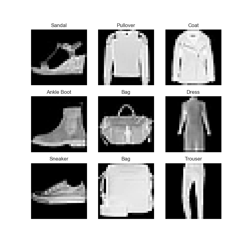
# data plotting
labels_map = {
0: "T-Shirt",
1: "Trouser",
2: "Pullover",
3: "Dress",
4: "Coat",
5: "Sandal",
6: "Shirt",
7: "Sneaker",
8: "Bag",
9: "Ankle Boot",
}
figure = plt.figure(figsize=(8, 8))
cols, rows = 3, 3
for i in range(1, cols * rows + 1):
sample_idx = torch.randint(len(train_data), size=(1,)).item()
img, label = train_data[sample_idx]
figure.add_subplot(rows, cols, i)
plt.title(labels_map[label])
plt.axis("off")
plt.imshow(img.squeeze(), cmap="gray")
plt.show()
Prepare Dataset With DataLoader
from torch.utils.data import DataLoader
train_dataloader = DataLoader(train_data, batch_size=64, shuffle=True)
test_dataloader = DataLoader(test_data, batch_size=64, shuffle=True)
# Now, each iteration can return a batch of train_features and train_labels
# As shuffle=True, after iterating over all batches the data is shuffled
train_features, train_labels = next(iter(train_dataloader))
train_features.size()
Out[319]: torch.Size([64, 1, 28, 28])
train_labels.size()
Out[320]: torch.Size([64])
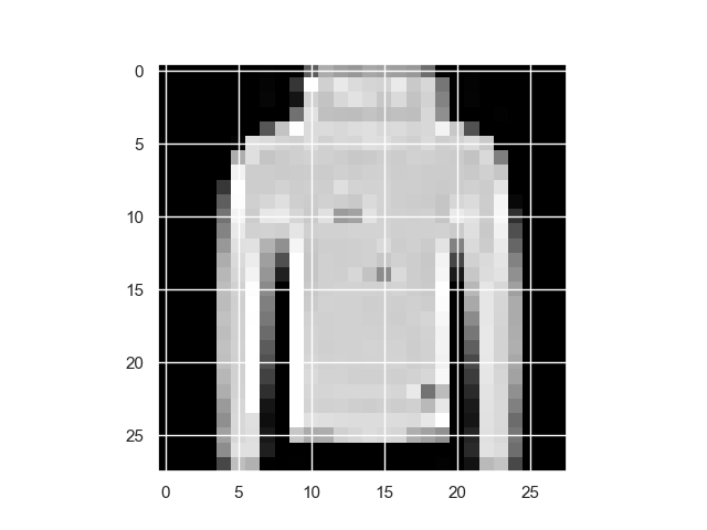
# plot the first image in the batch
img = train_features[0].squeeze()
label = train_labels[0]
plt.imshow(img, cmap="gray")
plt.show()
print(f"Label: {label}")
Transforms
Transforms are used to perform some manipulation of the data and make it suitable for training.
All TorchVision datasets have two parameters - transform to modify the features and target_transform to modify the labels. For FashionMINIST dataset, we can make the features into normalized tensors, and the labels into one-hot encoded tensors.
from torchvision.transforms import ToTensor, Lambda

train_data_tf = datasets.FashionMNIST(
    root="data",
    train=True,
    download=True,
    transform=ToTensor(),
    target_transform=Lambda(lambda y: torch.zeros(10, dtype=torch.float).scatter_(0, torch.tensor(y), value=1))
)
where Tensor.scatter_(dim, index, src, reduce=None) writes all values from the tensor src into self at the indices specified in the index tensor.
For example, data labeled 9 now turns into a 10 dimensional tensor with its final element being 1:
train_data[0][1]
Out[326]: 9

train_data_tf[0][1]
Out[327]: tensor([0., 0., 0., 0., 0., 0., 0., 0., 0., 1.])
Build the Neural Network
The torch.nn namespace provides all the building blocks to build neural networks. Every module in PyTorch subclasses the nn.Module.
import os
import torch
from torch import nn
from torch.utils.data import DataLoader
from torchvision import datasets, transforms

device = "cuda" if torch.cuda.is_available() else "cpu"
We define our neural network by subclassing nn.Module, and initialize the neural network layers in __init__. Then, nn.Module subclass implements the operations on input data in the forward method.
class NeuralNetwork(nn.Module):                 # subclass 'nn.Module'
    def __init__(self):
        super(NeuralNetwork, self).__init__()
        self.flatten = nn.Flatten()             # convert each 2D 28x28 image into a contiguous array of 784 pixel values
        self.linear_relu_stack = nn.Sequential( # nn.Sequential is an ordered container of modules.
            nn.Linear(28*28, 512),              # applies a linear transformation on the input using its stored weights and biases
            nn.ReLU(),
            nn.Linear(512, 512),
            nn.ReLU(),
            nn.Linear(512, 10),
        )

    def forward(self, x):
        x = self.flatten(x)
        logits = self.linear_relu_stack(x)
        return logits
Create an instance of NeuralNetwork, and move it to the device, and print its structure.
model = NeuralNetwork().to(device)
model
Out[333]:
NeuralNetwork(
  (flatten): Flatten(start_dim=1, end_dim=-1)
  (linear_relu_stack): Sequential(
    (0): Linear(in_features=784, out_features=512, bias=True)
    (1): ReLU()
    (2): Linear(in_features=512, out_features=512, bias=True)
    (3): ReLU()
    (4): Linear(in_features=512, out_features=10, bias=True)
  )
)
Finally, calling the model on the input returns a 10-dimensional tensor with raw predicted values for each class. We can further get the prediction probabilities by passing it through an instance of the nn.Softmax module.
logits = model(X)
pred_probab = nn.Softmax(dim=1)(logits)
y_pred = pred_probab.argmax(1)
Training Model
Training a model is an iterative process; in each iteration (called an epoch) the model makes a guess about the output, calculates the error in its guess (loss), collects the derivatives of the error with respect to its parameters, and optimizes these parameters using gradient descent.
For training, define the following hyperparameters:
learning_rate = 1e-3
batch_size = 64
epochs = 5
Common loss functions include nn.MSELoss (Mean Square Error) for regression tasks, and nn.NLLLoss (Negative Log Likelihood) for classification. nn.CrossEntropyLoss combines nn.LogSoftmax and nn.NLLLoss.
# Initialize the loss function
loss_fn = nn.CrossEntropyLoss()
All optimization logic is encapsulated in the optimizer object. Here, SGD optimizer is used; additionally, there are many different optimizers available in PyTorch such as ADAM and RMSProp.
optimizer = torch.optim.SGD(model.parameters(), lr=learning_rate)
Inside the training loop, there are three steps:
- Call
optimizer.zero_grad()to reset the gradients of model parameters. - Backpropagate the prediction loss with a call to
loss.backward(). - Call
optimizer.step()to adjust the parameters.
Full implementation:
def train_loop(dataloader, model, loss_fn, optimizer):
    size = len(dataloader.dataset)
    for batch, (X, y) in enumerate(dataloader):
        # Compute prediction and loss
        pred = model(X.to(device))
        loss = loss_fn(pred, y.to(device))

        # Backpropagation
        optimizer.zero_grad()
        loss.backward()
        optimizer.step()

        if batch % 100 == 0:
            loss, current = loss.item(), batch * len(X)
            print(f"loss: {loss:>7f}  [{current:>5d}/{size:>5d}]")

def test_loop(dataloader, model, loss_fn):
    size = len(dataloader.dataset)
    num_batches = len(dataloader)
    test_loss, correct = 0, 0

    with torch.no_grad():
        for X, y in dataloader:
            pred = model(X.to(device))
            test_loss += loss_fn(pred, y.to(device)).item()
            correct += (pred.argmax(1) == y.to(device)).type(torch.float).sum().item()

    test_loss /= num_batches
    correct /= size
    print(f"Test Error: \n Accuracy: {(100*correct):>0.1f}%, Avg loss: {test_loss:>8f} \n")
Finally, we are ready to train the model:
for t in range(epochs):
    print(f"Epoch {t+1}\n-------------------------------")
    train_loop(train_dataloader, model, loss_fn, optimizer)
    test_loop(test_dataloader, model, loss_fn)
print("Done!")
Save and Load the Model
PyTorch models store the learned parameters in an internal state dictionary, called state_dict. These can be persisted via the torch.save method:
import torchvision.models as models

model = models.vgg16(pretrained=True)
torch.save(model.state_dict(), 'model_weights.pth')
To load model weights, you need to create an instance of the same model first, and then load the parameters using load_state_dict() method.
model = models.vgg16() # we do not specify pretrained=True, i.e. do not load default weights
model.load_state_dict(torch.load('model_weights.pth'))
model.eval()
Alternately, we can also save and load the model together with the weights:
torch.save(model, 'model.pth')
model = torch.load('model.pth')
Complete Code
import os
import torch
from torch import nn
from torch.utils.data import Dataset
from torch.utils.data import DataLoader
from torchvision import datasets, transforms
from torchvision.transforms import ToTensor
import matplotlib.pyplot as plt

train_data = datasets.FashionMNIST(
    root="data",
    train=True,
    download=True,
    transform=ToTensor()
)

test_data = datasets.FashionMNIST(
    root="data",
    train=False,
    download=True,
    transform=ToTensor()
)

train_dataloader = DataLoader(train_data, batch_size=64, shuffle=True)
test_dataloader = DataLoader(test_data, batch_size=64, shuffle=True)

# =============================================================================
#
# =============================================================================
device = "cuda:0" if torch.cuda.is_available() else "cpu"

class NeuralNetwork(nn.Module):
    def __init__(self):
        super(NeuralNetwork, self).__init__()
        self.flatten = nn.Flatten()
        self.linear_relu_stack = nn.Sequential(
            nn.Linear(28*28, 512),
            nn.ReLU(),
            nn.Linear(512, 512),
            nn.ReLU(),
            nn.Linear(512, 10),
        )

    def forward(self, x):
        x = self.flatten(x)
        logits = self.linear_relu_stack(x)
        return logits

def train_loop(dataloader, model, loss_fn, optimizer):
    size = len(dataloader.dataset)
    for batch, (X, y) in enumerate(dataloader):
        # Compute prediction and loss
        pred = model(X.to(device))
        loss = loss_fn(pred, y.to(device))

        # Backpropagation
        optimizer.zero_grad()
        loss.backward()
        optimizer.step()

        if batch % 100 == 0:
            loss, current = loss.item(), batch * len(X)
            print(f"loss: {loss:>7f}  [{current:>5d}/{size:>5d}]")

def test_loop(dataloader, model, loss_fn):
    size = len(dataloader.dataset)
    num_batches = len(dataloader)
    test_loss, correct = 0, 0

    with torch.no_grad():
        for X, y in dataloader:
            pred = model(X.to(device))
            test_loss += loss_fn(pred, y.to(device)).item()
            correct += (pred.argmax(1) == y.to(device)).type(torch.float).sum().item()

    test_loss /= num_batches
    correct /= size
    print(f"Test Error: \n Accuracy: {(100*correct):>0.1f}%, Avg loss: {test_loss:>8f} \n")

# =============================================================================
#
# =============================================================================
model = NeuralNetwork().to(device)

learning_rate = 1e-3
batch_size = 64
epochs = 5

loss_fn = nn.CrossEntropyLoss()

optimizer = torch.optim.SGD(model.parameters(), lr=learning_rate)

for t in range(epochs):
    print(f"Epoch {t+1}\n-------------------------------")
    train_loop(train_dataloader, model, loss_fn, optimizer)
    test_loop(test_dataloader, model, loss_fn)
print("Done!")
Cuda Configuaration and Performance
- OS: Windows 10
- GPU: GTX 1660 Ti, 6.0 G
- Cuda: cuda_11.3.0_465.89
- CuDNN: Download cuDNN v8.2.1, for CUDA 11.x
- Pytorch: pip3 install torch==1.11.0+cu113 torchvision==0.12.0+cu113 torchaudio===0.11.0+cu113
- Comment: The same configuration works for Tensorflow 2.8
Run Without Cuda
It took 10.15 seconds to run a single epoch.
Epoch 1
-------------------------------
loss: 2.294270  [    0/60000]
loss: 2.301832  [ 6400/60000]
loss: 2.269578  [12800/60000]
loss: 2.261921  [19200/60000]
loss: 2.249367  [25600/60000]
loss: 2.231620  [32000/60000]
loss: 2.221365  [38400/60000]
loss: 2.215337  [44800/60000]
loss: 2.195395  [51200/60000]
loss: 2.163911  [57600/60000]
Test Error:
 Accuracy: 43.3%, Avg loss: 2.151954

Done!
Device: cpu  time: 10.152567199998884 s
Run With Cuda
It took 7.09 seconds to run a single epoch.
Epoch 1
-------------------------------
loss: 2.298946  [    0/60000]
loss: 2.289765  [ 6400/60000]
loss: 2.266071  [12800/60000]
loss: 2.248490  [19200/60000]
loss: 2.237693  [25600/60000]
loss: 2.221481  [32000/60000]
loss: 2.191885  [38400/60000]
loss: 2.181488  [44800/60000]
loss: 2.167980  [51200/60000]
loss: 2.151558  [57600/60000]
Test Error:
 Accuracy: 42.9%, Avg loss: 2.144230

Done!
Device: cuda:0  time: 7.088860100000602 s
Comments